Preface
本书并不是关于如何正确并且优雅的书写代码的,因为我假设你已经了解如何做到那些了。尽管本书有关于跟踪诊断,以便帮助你找到程序瓶颈和不必要的资源使用,以及性能调优的章节,但是,本书也不是真正的关于诊断和性能调优的书。
这两章是全书的最后部分,整本书都在为这些章节做准备。但是本书的真正目标是把所有的信息和细节展示出来,以便你真正的理解你的Erlang应用的性能表现。
关于本书
~~~~~
任何人期望:调整 Erlang 安装,了解如何调试 VM 崩溃,改进 Erlang 应用性能,深入理解 Erlang 如何工作,学习如何构建你自己的运行时环境
如果你想要调试VM,扩展 VM,调整性能,请跳到最后一章,但是想要真正理解那一章,你需要阅读这本书。
阅读方法
Erlang RunTime System (ERTS) 是一个有许多组件相互依赖的复杂系统。他使用了非常易于移植的方法编码,以便能够在从电脑棒到上TB内存的多核计算机上运行。为了能够为你的应用优化性能,你就不能只了解你的应用本身,同时需要深刻理解ERTS。
有了 ERTS 如何运行的知识,你就能够理解你的应用在 ERTS 之上运行的行为模式,也可以修补你应用的性能问题。在本书的第二部分,我们将深入介绍如何成功的运行,监控和扩展你的 ERTS 应用。
本书的读者不必是一位 Erlang 程序员,但需要对 Erlang 是什么有基本了解,接下来这段内容将给你一些关于 Erlang 的背景信息。
Erlang
本节中,我们将一起了解一些基础的 Erlang 概念,这对理解本书至关重要。
Erlang 被以它的发明人 Joe Armstrong 为代表的人称为一门面向并发的语言。并发在 Erlang 语言中处于核心地位,为了能够理解 Erlang 系统如何工作,你需要理解 Erlang 的并发模型。
首先,我们需要区分 “并发” 和 “并行”。本书中,“并发” 的概念是指2个或者更多的进程 能 相互独立的执行,这可以是先执行一个进程然后和其余进程交织执行,或者它们并行执行。提到 “并行” 执行时,我们是指多个进程在同一时刻使用多个物理执行单元执行。“并行”可能在不同层面上实现,例如通过单核的执行流水线的多个执行单元,通过CPU的多核芯,通过单一计算机的多个CPU,或者通过多个计算机实现。
Erlang 通过进程实现并发。从概念上讲,Erlang 的进程与大多数的操作系统进程类似,它们并行执行并且通过信号通信。但是实践上来说,Erlang 进程比绝大多数的操作系统进程都轻量,这是一个巨大的差异。在一些并发编程语言中,与 Erlang 进程对等的概念是 agents 。
Erlang 通过在 Erlang 虚拟机(BEAM)中交织的执行进程来达到并发的目的。在多核处理器上,BEAM 也可以通过运行在每个核心上运行一个调度器,在每个调度器上运行一个 Erlang 进程来实现并行,Erlang 系统的设计人员可以将系统分布在不同计算机上来达成更进一步的并行。
一个典型的 Erlang 系统(在 Erlang 中内置服务器或者服务)包含一定数量 Erlang 应用(application),对应于磁盘上的一个目录。每一个应用由若干 Erlang 模块(module)组成,模块对应于这个目录中的一些文件。每个模块包含若干函数(function),每个函数由若干表达式(expression)组成。
Erlang 是一个函数式语言,它没有语句,只有表达式。Erlang 表达式能被组合成 Erlang 函数。函数接受若干参数并且返回一个值。在 Erlang Code Examples 中,我们可以看到若干 Erlang 表达式和函数。
%% Some Erlang expressions:

true.
1+1.
if (X > Y) -> X; true -> Y end.

%% An Erlang function:

max(X, Y) ->
  if (X > Y) -> X;
     true    -> Y
  end.
Erlang VM 实现了许多 Erlang 内建函数 (built in functions 或 BIFs),这样做有效率方面的原因,例如 lists:append 的实现(它也可以在 Erlang 实现),同时也有在实现一些底层功能时, Erlang 本身较难实现的原因,例如 list_to_atom。
从 Erlang/OTP R13B03 版本开始,你也可以使用 C 语言和 Native Implemented Functions (NIF) 接口来实现自己的函数实现。
致谢
首先我要感谢 Ericsson OTP Team,感谢他们维护 Erlang 和 Erlang 运行时,并且耐心的回复我的提问。特别感谢Kenneth Lundin, Björn Gustavsson, Lukas Larsson, Rickard Green 和 Raimo Niskanen。
同时感谢本书的主要贡献者 Yoshihiro Tanaka, Roberto Aloi 和 Dmytro Lytovchenko,感谢 HappiHacking 和 TubiTV 对本书的赞助。
最后,感谢每一位编辑和修正本书的贡献者。
Yoshihiro Tanaka
Roberto Aloi
Dmytro Lytovchenko
Anthony Molinaro
Alexandre Rodrigues
Yoshihiro TANAKA
hitdavid
Ken Causey
Lukas Larsson
Kim Shrier
David
Trevor Brown
Andrea Leopardi
Anton N Ryabkov
Greg Baraghimian
Marc van Woerkom
Michał Piotrowski
Ramkumar Rajagopalan
Yves Müller
techgaun
Juan Facorro
Cameron Price
Kyle Baker
Buddhika Chathuranga
Luke Imhoff
fred
Alex Jiao
Milton Inostroza
PlatinumThinker
yoshi
Benjamin Tan Wei Hao
Alex Fu
Yago Riveiro
Antonio Nikishaev
Amir Moulavi
Eric Yu
Erick Dennis
Davide Bettio
tomdos
Jan Lehnardt
Chris Yunker
~~~~~
I: 理解 ERTS
1. Erlang 运行时系统介绍
Erlang 运行时系统(ERTS) 是一个有许多组件相互依赖的复杂系统。他使用了非常易于移植的方法编码,以便能够在从电脑棒到上TB内存的多核计算机上运行。为了能够为你的应用优化性能,你就不能只了解你的应用本身,同时需要深刻理解ERTS。
1.1. ERTS 和 Erlang 运行时系统
任何 Erlang 运行时系统 和 Erlang 运行时的特定实现系统有一点区别。由爱立信开发维护的 Erlang/OTP 是 Erlang 和 Erlang 运行时系统事实上的标准实现。在本书中,我将参考这个实现为 ERTS,将 Erlang RunTime System 中 T 字母大写 (See Section 1.3 for a definition of OTP)。
Erlang 运行时系统或者 Erlang 虚拟机并没有一个官方定义。你可以想象这样一个理想的柏拉图式系统看起来就像是ERTS,并且移除了所有特定实现细节。不幸的是,这是一个循环定义,因为你需要了解通用定义以便能够鉴别一个特定实现细节。在Erlang 的世界里,我们通常比较务实而不去担心这些。
我们将尝试使用术语 Erlang Runtime System 来指代 Erlang 运行时系统的一般的想法。反之,由 Ericsson 开发维护的特定实现被我们称为 Erlang 运行时系统或简称 ERTS.
Note 本书主要关于 ERTS,很小部分与通用 Erlang Runtime System 相关。你可以假设我们一直在基于 Ericsson 的实现讨论问题,除非我们明确声明我们在讨论通用原则。
1.2. 如何阅读本书
在本书的 Part II 部分,我们将关注如何为你的应用调整运行时系统,以及分析和调试你的应用和运行时系统。为了真正了解如何如何调整系统,你也需要了解系统。在本书的 Part I 部分,你讲深入理解运行时系统的工作原理。
在接下来 Part I 的章节中,我们将深入系统的各个组件。即使你并没有对全部组件有全面的理解,只要基本清楚每个组件是什么,也能够顺利阅读这些章节。剩余的介绍章节将向你介绍足够的基础信息和词汇术语,是你能够随意在这些章节之间切换阅读。
如果你有充裕时间,建议首次阅读按照顺序进行。有关 Erlang 和 ERTS 的词汇术语都在它们首次出现时解释。这样就可以在对某个特定组件有疑问时,使用 Part I 作为参考性的后续反复阅读。
1.3. ERTS
此处我们将对 ERTS 的主要组件以及一些词汇有一个概览,并在后续章节做更细节的描述。
1.3.1. Erlang 节点 (ERTS)
当你启动一个 Elixir / Erlang 应用或者系统,实际上你启动的是一个 Erlang 节点。这个节点运行了 ERTS 以及虚拟机 BEAM(或者也可能是其他的 Erlang 实现(参见 Section 1.4))
你的应用代码在 Erlang 节点上运行,节点的各层也同时对你的应用性能表现产生影响。我们来看一下组成节点的层次栈。这将帮你理解将你的系统运行在不同环境的选项。
使用OO的术语,可以说一个 Erlang 节点就是一个 Erlang 运行时系统类对象。在 Java 世界,等价的概念是 JVM 实例。
所有的 Elixir / Erlang 代码执行都在节点中完成。每个 Erlang 节点运行在一个操作系统进程中,在同一台计算机中可以同时运行多个 Erlang 节点。
根据 Erlang OTP 文档,一个节点实际上是一个命名的执行运行时系统。这样说来,如果你启动了 Elixir,但并没有通过命令行的以下开关来指定节点名字 --name NAME@HOST 或 --sname NAME (在 Erlang 运行时中是 -name 和 -sname ),你会启动一个运行时,但是不能叫节点。此时,函数 Node.alive? (在 Erlang 中为 is_alive()) 返回 false。
$ iex
Erlang/OTP 19 [erts-8.1] [source-0567896] [64-bit] [smp:4:4]
              [async-threads:10] [hipe] [kernel-poll:false]

Interactive Elixir (1.4.0) - press Ctrl+C to exit (type h() ENTER for help)
iex(1)> Node.alive?
false
iex(2)>
运行时系统 这个术语的使用并不严格。即使你并没有命名一个节点,也可以取得它的名字。在 Elixir 中,使用`Node.list` 参数 :this, 在 Erlang 中调用 `nodes(this).`即可:
iex(2)> Node.list :this
[:nonode@nohost]
iex(3)>
本书中,我们将使用术语 节点 来指代任何运行中的运行时实例,而不论它是否被命名。
1.3.2. 执行环境中的分层
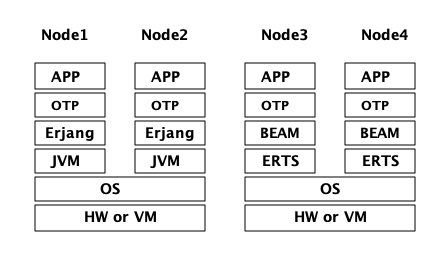
你的程序(应用)是在一个或者多个节点上运行的,它的性能不只取决于你的应用程序代码,同时取决于在 ERTS 栈 (ERTS stack)中,你应用以下的各层。图 Figure 1 中,你可以看到同一台计算机运行2个 Erlang 节点时的 ERTS 栈。
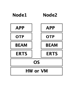
如果你用 Elixir,栈中还会有其他的层次。
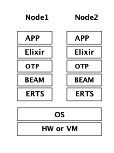
我们来观察栈中各层,看你如何为应用程序调优各层。
栈的最底部是程序运行依赖的硬件。改善你应用程序运行性能的最简单的方法是使用更好的硬件。如果因为经济、物理条件约束或者处于对环境问题的担忧等原因阻碍你升级硬件,你可能需要开始探索栈中的更高层次。
选择硬件的2个最主要考量是:它是否是多核系统,它是32位系统还是64位系统。计算机是否多核以及它是32/64位系统决定了你能够使用何种 ERTS 版本。
向上第二层是操作系统层。ERTS 能够在大多数的 Windows 和 包含 Linux, VxWorks, FreeBSD, Solaris, 以及 Mac OS X 的 POSIX “兼容” 系统上运行。如今,大部分的 ERTS 开发工作都是在 Linux 和 OS X 上完成的,所以你可以在这些平台上 ERTS 会有最佳的性能表现。Ericsson 一直以来在许多内部项目中使用 Solaris 平台,多年以来 ERTS 在 Solaris 上一直被调优。视你的使用场景,你也可能在 Solaris 上获得最佳性能。操作系统的选型往往被性能需求之外的因素约束。如果你在构建一个嵌入式应用,你可能需要选择 Raspbian (译注:树莓派系统)或者 VxWork,如果你在构建一些面向终端用户或者客户端的应用,你可能必须使用 Windows。ERTS 的 Windows 版本目前从性能和维护等方面来看,可能并不是最佳的选择,因为它不是最高优先级工作。如果你想使用一个64位版本的 ERTS ,你必须同时选择64位硬件和64位操作系统。本书并不会涉及到很多特定操作系统相关的问题,绝大多数例子假设你是在 Linux 系统上运行。
向上第三层是 Erlang 运行时系统,或者说是 ERTS 层。本层和向上第四层 — Erlang 虚拟机(BEAM)是本书的主要内容。
向上第五层 OTP 提供了 Erlang 标准库支持。OTP的原始含义是 “开放电信平台”(Open Telecom Platform),它包含了若干位构造类似电信交换等鲁棒的应用而提供构建模块的库(例如 supervisor, gen_server and gen_tcp)早期,这些随 ERTS 发布的其他标准库和 OTP 的含义是混杂的。现如今,大多数人将 OTP 和 Erlang 连用为 "Erlang/OTP" 指代 ERTS 以及由 Ericsson 发布的所有 Erlang 库。了解这些标准库并且清楚何时、如何使用它们可以极大地提高应用程序的性能。本书将不涉及任何关于标准库和OTP的细节,涉及这些方面书籍有很多。
如果你运行 Elixir 程序,第6层提供了 Elixir 环境和 Elixir 库。
最后,向上数第7层是你的应用程序以及其中使用的第三方库。应用层可以使用底层提供的所有功能。除了升级硬件,这也是你最容易实现应用性能优化的地方。在 Chapter 18 中介绍了一些诊断优化应用程序的提示和工具。在 Chapter 19 一章中,我们将了解如何找到应用崩溃的原因以及如何查找应用 bug。
有关如何构建运行 Erlang 节点的信息,请参见 Appendix A ,然后通过本书其余部分学习 Erlang 节点的组件知识。
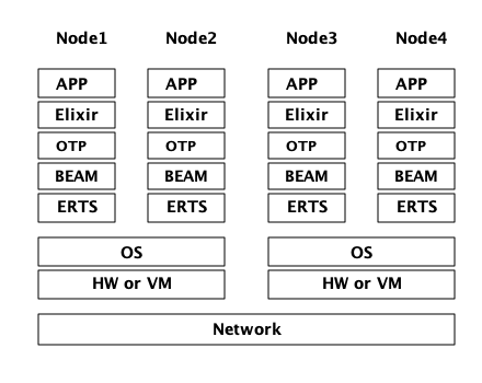
1.3.3. 分布式
Erlang 语言设计者的一个关键洞见是:为了构造一个可以 24小时 * 7天 工作的系统,你需要能够处理硬件失败。所以你需要至少将你的系统部署在2台以上的物理机器上。在每台机器上启动 Erlang 节点后,节点之间互相连接,跨节点的进程可以相互通信,就好像它们运行在同一个节点一样。
1.3.4. Erlang 编译器
Erlang 编译器负责将 Erlang 源代码从 .erl 文件编译为 BEAM 虚拟机代码。编译器本身就是使用 Erlang 编写的,它将自身编译为 BEAM 码,通常在运行的 Erlang 节点可用。为了引导运行时系统,包含编译器在内的数个预先编译好的 BEAM 文件都被放置在 bootstrap 目录。
有关编译器的更多信息可以参考 Chapter 2。
1.3.5. Erlang 虚拟机: BEAM
类似 JVM 是用来执行Java 代码的虚拟机一样,BEAM 是用来执行 Erlang 代码的虚拟机。BEAM 运行在 Erlang 节点上。
就像 ERTS 是 Erlang 运行时系统的更通用概念实现一样, BEAM 是 Erlang 虚拟机(EVM) 的一个通用实现。虽然没有对 EVM 组成结构的定义,但是 BEAM 的指令实际上分2层,分别是通用指令和特定指令。通用指令集可以看作是 EVM 的蓝图。
1.3.6. 进程
一个 Erlang 进程基本上与操作系统进程一样工作。每个进程拥有它自己的内存(mailbox, heap 和 stack)和带有进程信息的进程控制块(process control block , PCB)
所有的 Erlang 代码执行均在进程上下文中完成。一个 Erlang 节点可以拥有分多进程,这些进程可以通过消息传递或信号通信,如果多个节点是连接的,Erlang 进程也可以与其他节点上的进程通信。
想了解更多关于进程和 PCB 的知识,请参考 Chapter 3.
1.3.7. 调度器
调度器负责选择某个 Erlang 进程执行。通常来讲,调度器有2个队列,1个是 ready to run 的进程队列 ready queue ,另一个是等待接受消息的进程队列 waiting queue 。一个 waiting queue 中的进程如果收到了消息,或者接收超时,将被移动到 ready queue 。
调度器从 ready queue 中拿到第一个进程,并将它放到 BEAM 中执行一个_时间片_( time slice)。当时间片耗尽,BEAM会剥夺这个进程的执行,并把它放到 ready queue 的队尾。如果在时间片用尽前,这个进程被 receive 阻塞,他就会被放到 waiting queue 中。
Erlang 天生支持并发,这意味着从概念上讲,每一个进程与其他的进程同时执行,但是事实上,只有1个进程在虚拟机中运行。在多核系统中,Erlang 运行多个调度器,通常每核心一个,每个调度器独有自己的队列。这样 Erlang 获得了真正的并行能力。为了利用多核能力, ERTS 必须使用_SMP_ 被构建 (参见 Appendix A)。 SMP 意即_Symmetric MultiProcessing_,它意味着进程在多核中任意一个核心上运行的能力。
现实世界中,进程优先级等问题会使问题变得更复杂,等待队列使用时间轮实现。所有关于调度器的细节会在 Chapter 11中描述。
1.3.8. Erlang 标签方案
Erlang 是一个动态类型语言,运行时系统需要跟踪所有的数据对象的类型,这是通过标签方案(tagging scheme)完成的。每一个数据对象或指向数据对象的指针同时也会有一个带有其对象数据类型的标签。
一般来说,指针的一些位(bits)会被为标签预留,通过查找对象的标签的位模式(bit pattern),仿真器就可以确定他的数据类型。
这些标签在模式匹配、类型检测、原始操作(primitive operations)和垃圾收集是被使用。
Chapter 4 中完整的描述了标签方案。
1.3.9. 内存处理
Erlang 使用了自动内存管理方案,使得程序员不必担忧内存的分配和回收。每个进程都有可以按需扩容和缩容的堆和栈。
当一个进程出现堆空间不足时,虚拟机会首先尝试通过垃圾回收的方法回收并分配内存。垃圾收集器接下来会找到该进程的栈和堆,并将其中的活动数据复制到一个新的堆中,这样就扔掉了所有死数据。如果做完这些堆空间还是不够用,一个新的更大的堆会被分配出来,活动数据也会被移动到新的堆中。
关于当前的代际复制垃圾收集器的细节,包含被引用计数的 binary 处理,可以在 Chapter 12 章节中找到。
在使用 HiPE (High Performance Erlang ,译者注:类似 JIT ) 兼容本地代码的系统中,每个进程事实上有2个栈,1个 BEAM栈,1个本地代码栈,细节见 Chapter 17 。
1.3.10. 解释器和命令行接口
当你使用 erl 启动 Erlang 节点,可以得到一个命令行提示符。这就是 Erlang read eval print loop (REPL) 或者叫做 command line interface (CLI) 或简称 Erlang shell.
你可以在 Erlang 节点中输入并且在 shell 中直接执行。这种情况,代码不会被编译为 BEAM 码并被 BEAM执行,而是被 Erlang 解释器解析和解释执行。通常,解释后的代码与编译后的代码表现一致,但也存在一些差异,差异和其他方面的问题将在 Chapter 20 介绍。
1.4. 其他的 Erlang 实现
本书主要关注 Ericsson/OTP 实现的“标准” Erlang,即 ERTS。也有一些可用的其他 Erlang 实现,我们将在本节简要提及。
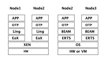
1.4.1. Erlang on Xen
Erlang on Xen (链接: http://erlangonxen.org,译注,网页已经没人维护) 是一个直接在服务器硬件上运行,中间没有操作系统层而只有一个 Xen 客户端薄层的 Erlang 实现。
这个运行在 Xen 上的虚拟机叫做 Ling,他同 BEAM 几乎100%二进制兼容。在 xref:the_eox_stack 中可以看到 Erlang 的 Xen 实现栈与 ERTS 的区别。需要注意的是,Xen 栈上的 Erlang 下没有操作系统。
Ling 实现了 BEAM 通用指令集,他可以重用 OTP 层的 BEAM 编译器来将 Erlang 编译成 Ling 代码。
1.4.2. Erjang
Erjang (链接: http://www.erjang.org,译注,项目已经废弃5年以上,最高支持Java 7) 是一个在 JVM 上运行的 Erlang 实现。它加载+.beam+ 文件后,将其重编译为 Java .class 文件。他与 BEAM 几乎 100% 二进制兼容。
图 xref:the_erjang_stack 中可以看到 Erlang 的 Erjang 实现栈与 ERTS 的区别。需要注意的是,这个方案中 JVM 替代了 BEAM 作为虚拟机,Erjang 在虚拟机上使用 Java 实现 ERTS 提供的服务。
现在,你应该对 ERTS 的各主要部分有了基本的了解,也了解了继续深入各组件所必须的词汇术语。如果你渴望了解某一个具体的组件,现在就可以跳到对应章节阅读了。或者你需要找一个特定问题的解决方案,你可以跳到 Part II 章节,尝试使用各种方法来调优、调试你的系统。
2. 编译器
虽然本书不是一本设计 Erlang 编程语言的书,但是,ERTS 的目标是运行 Erlang 代码,所以你需要了解如何编译 Erlang 代码。本章将涉及到用来生成可读的 BEAM 码的编译器选项,以及如何位生成的 beam 文件增加调试信息。本章的最后,也有一节关于 Elixir 编译器的内容。
那些对于将他们喜爱的语言编译为 ERTS 代码的读者,可以关注本章包含的关于编译器中的中间格式区别的详情,以及如何在 beam 编译器后台挂载你的编译器的信息。
我会展示解析转换,并通过样例来说明如何通过它们来调整 Erlang 语言。
2.1. 编译 Erlang
Erlang 被从 .erl 格式文件的模块源代码,编译成二进制 .beam 文件
编译器可以从操作系统终端,通过 erlc 启动:
> erlc foo.erl编译器也可以在 Erlang 终端中,使用 c 或者调用 compile:file/{1,2} 来调用。
1> c(foo).或者
1> compile:file(foo).compile:file 的第二个可选参数接受编译器选项 list。全部的可选参数清单可以在编译器模块的文档中找到,参见 http://www.erlang.org/doc/man/compile.html 。
通常,编译器会将 Erlang 源代码从 .erl 格式文件,编译并写入到二进制 .beam 文件中。你也可以通过使用编译器的 binary 选项,将编译二进制结果作为Erlang 项式(Erlang term)直接输出。这个选项被重载以用来使用数据来返回中间格式结果,而不是将其写入文件。如果你期望编译器返回Core Erlang 代码,可以使用 [core, binary] 选项。
编译器的执行,包含由如图 Figure 6 中所示的若干“遍”(pass)。
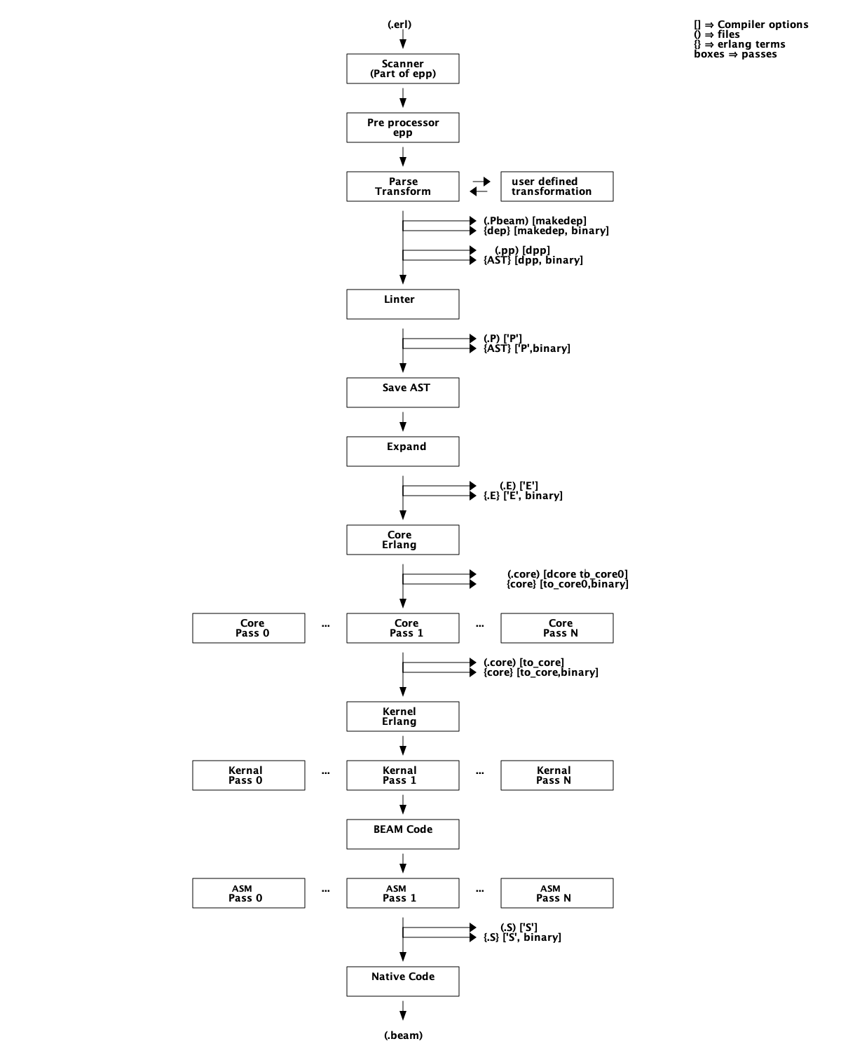
如果你想看到完整且最新的编译器的“遍”清单,可以在 Erlang 终端中运行 compile:options/0。当然,有关浏览器的最终信息来源来自于 compile.erl
2.2. 产生中间结果输出
阅读由编译器产生的代码对于试图理解虚拟机如何工作有很大帮助。幸运的是,编译器可以输出每遍后产生的中间代码,以及最终的 beam 码。
我们来尝试一下这些新知识,并且观察一下生成的代码。
 1> compile:options().
 dpp - Generate .pp file
 'P' - Generate .P source listing file
...
'E' - Generate .E source listing file
...
'S' - Generate .S file
我们来尝试一个小例子程序 "world.erl":
-module(world).
-export([hello/0]).

-include("world.hrl").

hello() -> ?GREETING.
以及包含文件: "world.hrl"
-define(GREETING, "hello world").如果此时使用 'P' 选项编译以得到解析后的文件,你会得到一个 "world.P" 文件。
2> c(world, ['P']).
** Warning: No object file created - nothing loaded **
ok
在结果输出的 .P 文件中,你可以看到应用预处理器(解析转换)处理后的美化格式版本的代码:
-file("world.erl", 1).

-module(world).

-export([hello/0]).

-file("world.hrl", 1).

-file("world.erl", 4).

hello() ->
    "hello world".
要查看所有的源代码转换执行完毕后代码的样子,可以使用 'E' 选项。
3> c(world, ['E']).
** Warning: No object file created - nothing loaded **
ok
这将输出一个 .E 文件,其中所有的编译器指令都被移除,并且内建函数 module_info/{1,2} 也被加入到源代码中。
-vsn("\002").

-file("world.erl", 1).

-file("world.hrl", 1).

-file("world.erl", 5).

hello() ->
    "hello world".

module_info() ->
    erlang:get_module_info(world).

module_info(X) ->
    erlang:get_module_info(world, X).
我们将在观察 Section 2.3.2 解析转换时,使用 'P' 和 'E' 选项,但首先我们先来看看汇编器生成的 BEAM 码。使用编译器选项 'S' 可以得到一个内容为源代码对应的每条 BEAM 指令的 Erlang 项式的 .S 文件。
3> c(world, ['S']).
** Warning: No object file created - nothing loaded **
ok
world.S 文件看起来是这样的:
{module, world}.  %% version = 0

{exports, [{hello,0},{module_info,0},{module_info,1}]}.

{attributes, []}.

{labels, 7}.


{function, hello, 0, 2}.
  {label,1}.
    {line,[{location,"world.erl",6}]}.
    {func_info,{atom,world},{atom,hello},0}.
  {label,2}.
    {move,{literal,"hello world"},{x,0}}.
    return.


{function, module_info, 0, 4}.
  {label,3}.
    {line,[]}.
    {func_info,{atom,world},{atom,module_info},0}.
  {label,4}.
    {move,{atom,world},{x,0}}.
    {line,[]}.
    {call_ext_only,1,{extfunc,erlang,get_module_info,1}}.


{function, module_info, 1, 6}.
  {label,5}.
    {line,[]}.
    {func_info,{atom,world},{atom,module_info},1}.
  {label,6}.
    {move,{x,0},{x,1}}.
    {move,{atom,world},{x,0}}.
    {line,[]}.
    {call_ext_only,2,{extfunc,erlang,get_module_info,2}}.
因为这是一个由点 (".",译者注:点是每行的结尾) 分隔的 Erlang 项式组成的文件,你可以使用如下命令将这个文件读入 Erlang 终端:
{ok, BEAM_Code} = file:consult("world.S").
汇编码大部分按照原始的源代码格式布局。首条指令定义了代码模块的名称。注释中提到的版本(%% version = 0) 是 beam 操作码格式的版本(由 beam_opcodes 给出的 beam_opcodes:format_number/0) 接下来是一个导出清单以及编译器属性(本例中没有),这和 Erlang 源码模块中的差不多。 第一条像是 beam 指令的是 {labels, 7} ,它告诉虚拟机代码中共有7个标签(label),使得对代码的一遍处理即可为所有的标签分配空间。 接下来是每个函数的实际代码。第一条指令给出了函数名称,标签数表示的参数个数和入口点。 你可以使用 'S' 选项来尽最大努力使你理解 BEAM 如何工作,我们也将在后续章节这么做。当你开发自己的编程语言,通过Core Erlang 编译为 BEAM 码时,能看到生成的代码也是非常有价值的。
2.3. 编译器的遍(Pass)
接下来几节,我们将深入到图 Figure 6 中所示的编译器的各遍。对于面向 BEAM 的编程语言设计者,这些内容将向你展示使用 宏(macros),解析转换(parse transforms),Core Erlang,BEAM 码等不同方法你可以做什么,以及它们之间是如何相互依赖的。 在调优 Erlang 代码时,通过查看优化前后的生成代码,来了解何种优化在何时,以何种方式起作用是非常有效的。
2.3.1. 编译器 Pass: Erlang 预处理器 (epp)
编译过程起始于一个组合的分词器(或者扫描器)和预处理器。预处理器驱动分词器运行。这意味着宏被以符号的方式展开,而不纯粹是字符串替换(不像是 m4 或 cpp)。你不能够使用 Erlang 宏来定义自己的语法,宏像一个与周围字符独立的符号一样被展开。所以你也不能将一个宏与(它前后连续的)字符连接为新的符号:
-define(plus,+).
t(A,B) -> A?plus+B.
This will expand to
t(A,B) -> A + + B.
and not
t(A,B) -> A ++ B.
另一方面,由于宏展开实在符号级别完成的,宏的右值(rhs)也不必是一个合法的 Erlang 项式,例如:
-define(p,o, o]).
 t() -> [f,?p.
这除了能帮你赢得 Erlang 混乱代码大赛之外,没什么真实用处。记住这个知识的主要用途是,你不能使用 Erlang 预处理器来定义一个与 Erlang 句法不同的编程语言。幸运的是,你可以用其他手段定义新语言,我们将在后文看到这些内容。
2.3.2. 编译器 Pass: 解析转换(Parse Transformations)
调整Erlang语言最简单的方法是通过解析转换(Parse Transformations 或 parse transforms)。解析转换带有各种各样的警告,比如OTP文档中的注释:
| Programmers are strongly advised not to engage in parse transformations and no support is offered for problems encountered. |
当你使用了解析转换,你基本上在写一个额外的编译器“pass”,如果不小心的话,可能会导致意外的结果。你需要在使用解析转换的模块声明对它的使用,这对模块来说是本地的,这样对编译器的调整也比较安全。在我看来,应用解析转换最大的问题在于你自己发明的句法,这可能对别人阅读代码造成许多困难。至少在你的解析转换与广受欢迎的 QLC 等齐名前都如此。
好吧,所以你知道你不应该使用它,但如果你必须使用,你得知道它是什么。解析转换是在抽象语法树(AST)(参见 http://www.erlang.org/doc/apps/erts/absform.html)上运行的函数。编译器依次做预处理,符号化和解析,然后它会用 AST 调用解析转换函数,并期望返回新的AST。
这意味着您不能从根本上改变 Erlang 句法,但是您可以更改语义。举个例子,假如你想在 Erlang 代码中直接写json代码,你也很幸运,因为 json 和 Erlang 的标记是基本上是一样的。另外,由于 Erlang 编译器在解析转换后的 linter pass 才会做大部分的完整性检查工作,所以,可以允许一个不代表有效Erlang的 AST。
要编写解析转换,您需要编写一个Erlang模块(让我们称它为_p_),它导出函数+parse_transform/2+。如果这个模块(我们称其为_m_)的编译过程包含 + {parse_transform p} + 编译器选项,这个函数就会在解析转换 pass 期间被编译器调用。函数的参数是模块 m 的 AST 和调用的编译器时的编译器选项。
|
注意,您不能从文件中给出的任何编译器选项。因为你不能够从代码来给出(编译器)选项,还真有点麻烦。 编译器直到发生在解析转换后的 expand pass才会展开编译器选项。 |
抽象格式的文档确实有些密集,我们很难通过阅读来掌握抽象格式文档。我鼓励您使用句法工具(syntax_tools),特别是 erl_syntax_lib 用于处理AST上的任何重要工作。
在这里,为帮助我们理解,我们将开发一个简单的解析转换例子来理解AST。我们将直接在 AST 上工作,使用老的可靠的 io:format 方法来代替句法工具(syntax_tools)。
首先,我们创建一个可以编译 json_test.erl 的例子:
-module(json_test).
-compile({parse_transform, json_parser}).
-export([test/1]).

test(V) ->
    <<{{
      "name"  : "Jack (\"Bee\") Nimble",
      "format": {
                 "type"      : "rect",
                 "widths"     : [1920,1600],
                 "height"    : (-1080),
                 "interlace" : false,
                 "frame rate": V
                }
      }}>>.
然后,我们创建一个最小化的解析转换模块 json_parser.erl :
-module(json_parser).
-export([parse_transform/2]).

parse_transform(AST, _Options) ->
  io:format("~p~n", [AST]),
  AST.
这个有代表性的解析转换返回了未经改变的 AST,同时将其打印出来,这样你可以观察 AST 到底是什么样子的。
> c(json_parser).
{ok,json_parser}
2> c(json_test).
[{attribute,1,file,{"./json_test.erl",1}},
 {attribute,1,module,json_test},
 {attribute,3,export,[{test,1}]},
 {function,5,test,1,
  [{clause,5,
    [{var,5,'V'}],
    [],
    [{bin,6,
      [{bin_element,6,
        {tuple,6,
         [{tuple,6,
           [{remote,7,{string,7,"name"},{string,7,"Jack (\"Bee\") Nimble"}},
            {remote,8,
             {string,8,"format"},
             {tuple,8,
              [{remote,9,{string,9,"type"},{string,9,"rect"}},
               {remote,10,
                {string,10,"widths"},
                {cons,10,
                 {integer,10,1920},
                 {cons,10,{integer,10,1600},{nil,10}}}},
               {remote,11,{string,11,"height"},{op,11,'-',{integer,11,1080}}},
               {remote,12,{string,12,"interlace"},{atom,12,false}},
               {remote,13,{string,13,"frame rate"},{var,13,'V'}}]}}]}]},
        default,default}]}]}]},
 {eof,16}]
./json_test.erl:7: illegal expression
./json_test.erl:8: illegal expression
./json_test.erl:5: Warning: variable 'V' is unused
error
因为模块包含无效的 Erlang 语法,故编译+json_test+失败,但是你可以看到AST是什么样子的。现在我们可以编写一些函数来遍历 AST 并将 json 代码回写到 Erlang 代码中。[1]
-module(json_parser).
-export([parse_transform/2]).

parse_transform(AST, _Options) ->
    json(AST, []).

-define(FUNCTION(Clauses), {function, Label, Name, Arity, Clauses}).

%% We are only interested in code inside functions.
json([?FUNCTION(Clauses) | Elements], Res) ->
    json(Elements, [?FUNCTION(json_clauses(Clauses)) | Res]);
json([Other|Elements], Res) -> json(Elements, [Other | Res]);
json([], Res) -> lists:reverse(Res).

%% We are interested in the code in the body of a function.
json_clauses([{clause, CLine, A1, A2, Code} | Clauses]) ->
    [{clause, CLine, A1, A2, json_code(Code)} | json_clauses(Clauses)];
json_clauses([]) -> [].


-define(JSON(Json), {bin, _, [{bin_element
                                         , _
                                         , {tuple, _, [Json]}
                                         , _
                                         , _}]}).

%% We look for: <<"json">> = Json-Term
json_code([])                     -> [];
json_code([?JSON(Json)|MoreCode]) -> [parse_json(Json) | json_code(MoreCode)];
json_code(Code)                   -> Code.

%% Json Object -> [{}] | [{Label, Term}]
parse_json({tuple,Line,[]})            -> {cons, Line, {tuple, Line, []}};
parse_json({tuple,Line,Fields})        -> parse_json_fields(Fields,Line);
%% Json Array -> List
parse_json({cons, Line, Head, Tail})   -> {cons, Line, parse_json(Head),
                                                       parse_json(Tail)};
parse_json({nil, Line})                -> {nil, Line};
%% Json String -> <<String>>
parse_json({string, Line, String})     -> str_to_bin(String, Line);
%% Json Integer -> Intger
parse_json({integer, Line, Integer})   -> {integer, Line, Integer};
%% Json Float -> Float
parse_json({float, Line, Float})       -> {float, Line, Float};
%% Json Constant -> true | false | null
parse_json({atom, Line, true})         -> {atom, Line, true};
parse_json({atom, Line, false})        -> {atom, Line, false};
parse_json({atom, Line, null})         -> {atom, Line, null};

%% Variables, should contain Erlang encoded Json
parse_json({var, Line, Var})         -> {var, Line, Var};
%% Json Negative Integer or Float
parse_json({op, Line, '-', {Type, _, N}}) when Type =:= integer
                                             ; Type =:= float ->
                                          {Type, Line, -N}.
%% parse_json(Code)                  -> io:format("Code: ~p~n",[Code]), Code.

-define(FIELD(Label, Code), {remote, L, {string, _, Label}, Code}).

parse_json_fields([], L) -> {nil, L};
%% Label : Json-Term  --> [{<<Label>>, Term} | Rest]
parse_json_fields([?FIELD(Label, Code) | Rest], _) ->
    cons(tuple(str_to_bin(Label, L), parse_json(Code), L)
         , parse_json_fields(Rest, L)
         , L).


tuple(E1, E2, Line)    -> {tuple, Line, [E1, E2]}.
cons(Head, Tail, Line) -> {cons, Line, Head, Tail}.

str_to_bin(String, Line) ->
    {bin
     , Line
     , [{bin_element
         , Line
         , {string, Line, String}
         , default
         , default
        }
       ]
    }.
现在,我们可以无错的将 json_test 编译通过了:
1> c(json_parser).
{ok,json_parser}
2> c(json_test).
{ok,json_test}
3> json_test:test(42).
[{<<"name">>,<<"Jack (\"Bee\") Nimble">>},
{<<"format">>,
  [{<<"type">>,<<"rect">>},
   {<<"widths">>,[1920,1600]},
   {<<"height">>,-1080},
   {<<"interlace">>,false},
   {<<"frame rate">>,42}]}]
由 parse_transform/2 产生的 AST 必须是合法的 Erlang 代码,除非是你做多个解析转换。(译注:指多次解析转换的中间结果AST),代码的合法性检查是在下边的编译 pass 进行的。
2.3.3. 编译器 Pass: Linter
Linter 为句法正确但是不好的代码生成警告,类似"export_all flag enabled"
2.3.4. 编译器 Pass: 保存抽象语法树(AST)
为了启用对某模块的调试,您可以“调试编译”该模块,即将选项 debug_info 传递给编译器。抽象语法树将被“Save AST”保存,直到编译结束时,它将被写入.beam文件。
重要的是,要注意代码是在任意优化被应用前保存的,所以如果编译器的优化 pass 有 bug,你将在调试器中运行代码时得到不同的行为。如果你正在实现你自己的编译器这可能会把你搞糊涂。
2.3.5. 编译器 Pass: Expand
在扩展(Expand)阶段,诸如 record 等源 erlang 结构将被扩展为底层的 erlang 结构。编译器选项 "-compile(...)" 也会被 扩展 为元数据。
2.3.6. 编译器 Pass: Core Erlang
Core Erlang 是一种适用于编译器优化的严格函数式语言。通过减少表示同一操作的方法的数量,使代码转换更容易。其中一种方法是通过引入 let 和 letrec 表达式来使作用域更明确。
核心Erlang是一种适用于编译器优化的严格函数式语言。通过减少表示同一操作的方法的数量,使代码转换更容易。其中一种方法是通过引入 let 和 letrec 表达式来使作用域更明确。
对于希望在 ERTS 中运行的语言来说,Core Erlang 是最好的目标。它很少更改,并且以一种干净的方式包含了 Erlang 的所有方面。如果您直接针对beam指令集,您将不得不处理更多的细节,并且该指令集通常在每个主要的ERTS版本之间略有变化。另一方面,如果您直接以Erlang为目标,那么您可以描述的内容将受到更大的限制,而且您还必须处理更多的细节,因为 Core Erlang 是一种更干净的语言。
你可以使用 “to_core” 选项来将 Erlang 文件编译为 core erlang,但请注意,这将把 Core Erlang 程序写入带有 “.core" 扩展名的文件。你可以通过编译器选项 "from_core" 来编译来自带有 “.core" 扩展名的 core erlang 文件。
1> c(world, to_core).
** Warning: No object file created - nothing loaded **
ok
2> c(world, from_core).
{ok,world}
注意 .core 文件是用人类可读的 core 格式编写的文本文件。要获得作为 Erlang 项式的核心程序,可以在编译中添加+binary+选项。
2.3.7. 编译器 Pass: Kernel Erlang
Kernel Erlang 是 Core Erlang 的一个扁平版本,它们有一些不同之处。例如,每个变量在一个完整的函数作用域中都是唯一的。模式匹配被编译成更原始的操作。
2.3.8. 编译器 Pass: BEAM 码
正常编译的最后一步是外部 beam 码格式。一些底层的优化,如死代码块消除和窥孔优化是在这个级别上完成的。
BEAM 码在 Chapter 7 和 Appendix B 中有详细描述。
2.3.9. 编译器 Pass: 本地(Native)码
如果您在编译中添加了 native 标志,并且您有一个启用了 HiPE (High Performance Erlang ,译者注:类似 JIT ) 的运行时系统,那么编译器将为您的模块生成本机代码,并将本地代码与 beam 代码一起存储在 .beam 文件中。
2.4. 其他编译器工具
有许多工具可以帮助您处理代码生成和代码操作。这些工具是用 Erlang 编写的,但并不是运行时系统的一部分,但是如果你想在 BEAM 之上实现另一种语言,了解它们是非常好的。
在本节中,我们将介绍三个最有用的代码工具: 词法分析器 (Leex)、解析器生成器(Yecc),和一组用于操作(语言)抽象形式的通用函数(Syntax Tools)。
2.4.1. Leex
Leex是Erlang 词法分析器生成器。词法分析器生成器从定义文件 xrl 获取 DFA (译注,DFA 是 Deterministic Finite Automaton 的简称,形式语言术语,译为 确定有限自动机)的描述,并生成一个与 DFA 描述的符号相匹配 Erlang 程序。
关于如何为分词器编写 DFA 定义的细节已经超出了本书的范围。要得到详细的解释,我推荐 “龙书”。(是指 Aho, Sethi 和 Ullman合著的 《Compiler》)。其他好的资源包括激发了 leex 灵感的 “flex” 程序的手册,以及 leex 文档本身。如果你已经安装了 flex,你可以通过输入以下命令来阅读完整的手册:
> info flex
在线 Erlang 文档也有 leex 手册 (参见 yecc.html)。
我们可以使用词法分析器生成器创建一个识别 JSON 符号的 Erlang 程序。通过查看JSON定义 link:http://www.ecma-international.org/publications/files/ECMA-ST/ECMA-404.pdf 我们可以看到,我们只需要处理少量的令牌。
Definitions.

Digit         = [0-9]
Digit1to9     = [1-9]
HexDigit      = [0-9a-f]
UnescapedChar = [^\"\\]
EscapedChar   = (\\\\)|(\\\")|(\\b)|(\\f)|(\\n)|(\\r)|(\\t)|(\\/)
Unicode       = (\\u{HexDigit}{HexDigit}{HexDigit}{HexDigit})
Quote         = [\"]
Delim         = [\[\]:,{}]
Space         = [\n\s\t\r]

Rules.

{Quote}{Quote} : {token, {string, TokenLine, ""}}.
{Quote}({EscapedChar}|({UnescapedChar})|({Unicode}))+{Quote} :
  {token, {string, TokenLine, drop_quotes(TokenChars)}}.

null  : {token, {null,  TokenLine}}.
true  : {token, {true,  TokenLine}}.
false : {token, {false, TokenLine}}.

{Delim} : {token, {list_to_atom(TokenChars), TokenLine}}.

{Space} : skip_token.

-?{Digit1to9}+{Digit}*\.{Digit}+((E|e)(\+|\-)?{Digit}+)? :
  {token, {number, TokenLine, list_to_float(TokenChars)}}.
-?{Digit1to9}+{Digit}* :
  {token, {number, TokenLine, list_to_integer(TokenChars)+0.0}}.

Erlang code.
-export([t/0]).

drop_quotes([$" | QuotedString]) -> literal(lists:droplast(QuotedString)).
literal([$\\,$" | Rest]) ->
  [$"|literal(Rest)];
literal([$\\,$\\ | Rest]) ->
  [$\\|literal(Rest)];
literal([$\\,$/ | Rest]) ->
  [$/|literal(Rest)];
literal([$\\,$b | Rest]) ->
  [$\b|literal(Rest)];
literal([$\\,$f | Rest]) ->
  [$\f|literal(Rest)];
literal([$\\,$n | Rest]) ->
  [$\n|literal(Rest)];
literal([$\\,$r | Rest]) ->
  [$\r|literal(Rest)];
literal([$\\,$t | Rest]) ->
  [$\t|literal(Rest)];
literal([$\\,$u,D0,D1,D2,D3|Rest]) ->
  Char = list_to_integer([D0,D1,D2,D3],16),
  [Char|literal(Rest)];
literal([C|Rest]) ->
  [C|literal(Rest)];
literal([]) ->[].

t() ->
  {ok,
   [{'{',1},
    {string,2,"no"},
    {':',2},
    {number,2,1.0},
    {'}',3}
   ],
   4}.
通过使用 Leex 编译器,我们可以将这个 DFA 编译为 Erlang 代码,并且通过提供 dfa_graph 选项,我们还可以生成一个 dot-file,可以用 Graphviz 查看。
1> leex:file(json_tokens, [dfa_graph]).
{ok, "./json_tokens.erl"}
2>
你可以通过 dotty 来查看 DFA 图。
> dotty json_tokens.dot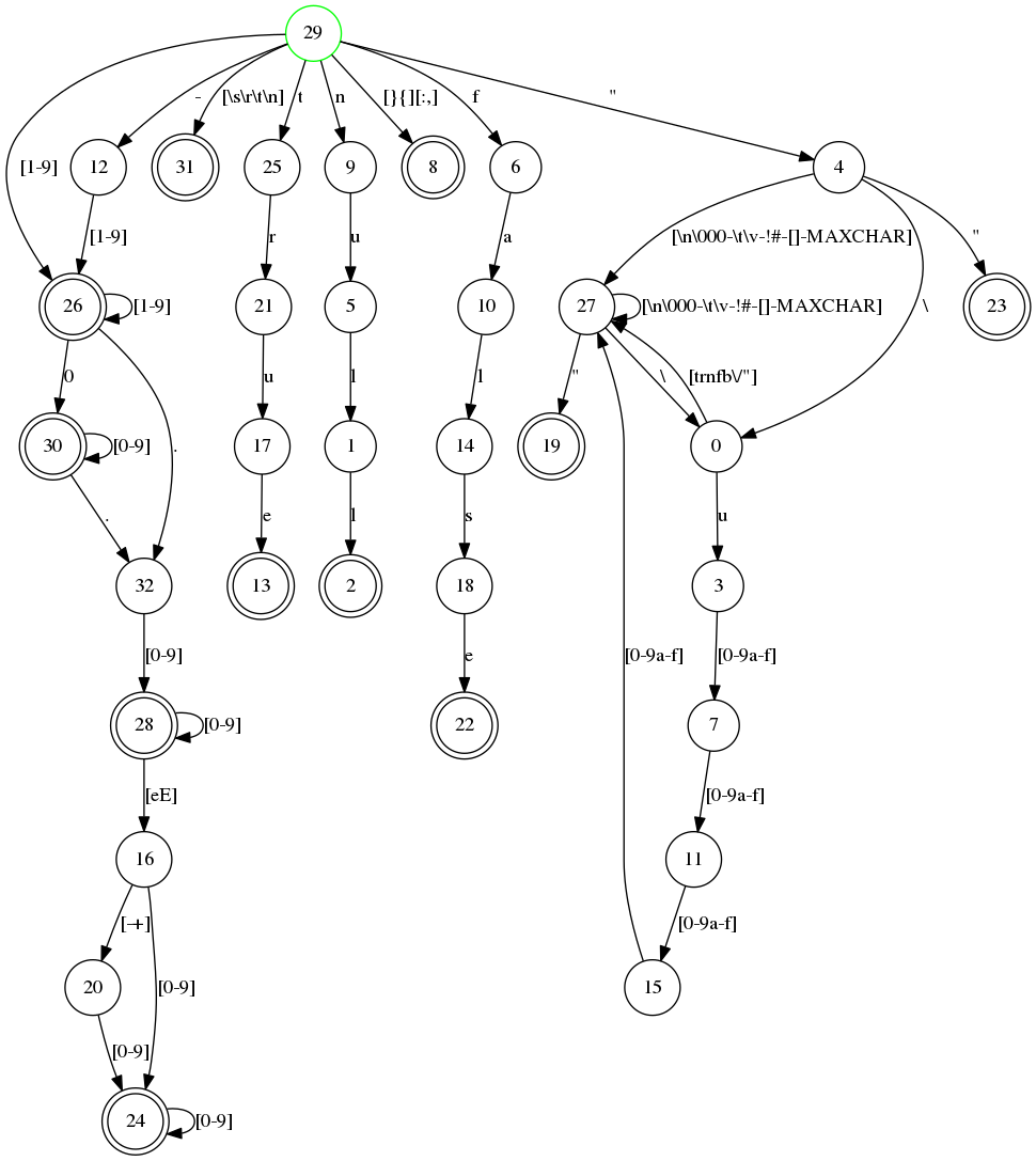
我们可以在示例 json 文件 (test.json) 上尝试分词器。
{
    "no" : 1,
    "name"  : "Jack \"Bee\" Nimble",
    "escapes" : "\b\n\r\t\f\//\\",
    "format": {
        "type"      : "rect",
        "widths"    : [1920,1600],
        "height"    : -1080,
        "interlace" : false,
        "unicode"   : "\u002f",
        "frame rate": 4.5
    }
}
首先,我们需要编译分词器,然后读取文件并将其转换为字符串。最后,我们可以使用 leex 生成的 string/1 函数来将测试文件分词。
2> c(json_tokens).
{ok,json_tokens}.
3> f(File), f(L), {ok, File} = file:read_file("test.json"), L = binary_to_list(File), ok.
ok
4> f(Tokens), {ok, Tokens,_} = json_tokens:string(L), hd(Tokens).
{'{',1}
5>
shell 函数 f/1 告诉终端忘记变量绑定。如果您想尝试多次绑定变量的命令,例如在编写 lexer 并希望在每次重写后尝试它的场景下,这是很有用的。有关 shell 命令的细节将在后面的章节中介绍。
有了 JSON 的分词器,我们现在可以使用解析器生成器 Yecc 来编写一个 JSON 解析器了。
2.4.2. Yecc
Yecc 是 Erlang 的解析器生成器。该名称来自Yacc (Yet another compiler compiler),它是 C 的经典的解析器生成器。
现在我们有了一个用于 JSON 项式的词法分析器,我们就可以使用 yecc 编写一个解析器。
Nonterminals value values object array pair pairs.

Terminals number string true false null '[' ']' '{' '}' ',' ':'.

Rootsymbol value.

value -> object  :  '$1'.
value -> array   :  '$1'.
value -> number  :  get_val('$1').
value -> string  :  get_val('$1').
value -> 'true'  :  get_val('$1').
value -> 'null'  :  get_val('$1').
value -> 'false' :  get_val('$1').

object -> '{' '}' : #{}.
object -> '{' pairs '}' : '$2'.

pairs -> pair : '$1'.
pairs -> pair ',' pairs : maps:merge('$1', '$3').

pair -> string ':' value : #{ get_val('$1') => '$3' }.

array -> '[' ']' : {}.
array -> '[' values ']' : list_to_tuple('$2').

values -> value : [ '$1' ].
values -> value ',' values : [ '$1' | '$3' ].


Erlang code.

get_val({_,_,Val}) -> Val;
get_val({Val, _}) -> Val.
然后,我们可以使用 yecc 生成一个实现解析器的 Erlang 程序,并调用 parse/1 函数,该函数使用由分词器生成的记号作为参数。
5> yecc:file(yecc_json_parser), c(yecc_json_parser).
{ok,yexx_json_parser}
6> f(Json), {ok, Json} = yecc_json_parser:parse(Tokens).
{ok,#{"escapes" => "\b\n\r\t\f////",
      "format" => #{"frame rate" => 4.5,
        "height" => -1080.0,
        "interlace" => false,
        "type" => "rect",
        "unicode" => "/",
        "widths" => {1920.0,1.6e3}},
       "name" => "Jack \"Bee\" Nimble",
       "no" => 1.0}}
当您希望将自己的完整语言编译到 Erlang 虚拟机时,Leex 和 Yecc 工具非常适合。通过将它们与语法工具 (特别是 Merl ) 结合使用,您可以操作 Erlang 抽象语法树,以生成 Erlang 代码或更改 Erlang 代码的行为。
2.5. 语法工具和 Merl
语法工具是一组库,用于操作 Erlang 抽象语法树 (AST) 的内部表示。
语法工具应用程序还包括自 Erlang 18.0 以来的工具 Merl。你可以使用 Merl 来非常容易地操作语法树,并用 Erlang 代码编写解析转换。
您可以在 Erlang.org 站点上找到语法工具的文档 http://erlang.org/doc/apps/syntax_tools/chapter.html。
2.6. 编译 Elixir
在 Beam 上编写自己的编程语言的另一种方法,是使用 Elixir 中的元编程工具。Elixir 通过 Erlang 抽象语法树编译 Beam 代码。
使用 Elixir 的 defmacro,您可以直接在 Elixir 中定义您自己的领域特定语言(DSL)。
3. 进程
轻量级进程的概念是 Erlang 和 BEAM 的本质;它使 BEAM 从其他虚拟机中脱颖而出。为了理解 BEAM (以及 Erlang 和 Elixir )是如何工作的,您需要了解进程是如何工作的细节,这将帮助您理解 BEAM 的核心概念,包括对进程来说什么是容易且低成本的,什么是困难且昂贵的。
BEAM 中的几乎所有内容都与进程的概念有关,在本章中,我们将进一步了解这些关系。我们将对 Chapter 1 部分的内容进行扩展,并更深入地了解一些概念,如内存管理、消息传递,特别是调度。
Erlang 进程与操作系统进程非常相似。它有自己的地址空间,它可以通过信号和消息与其他进程通信,并且执行是由抢占式调度程序控制的。
当你的 Erlang 或 Elixir 系统中出现性能问题时,这个问题通常是由特定进程中的问题或进程之间的不平衡引起的。当然还有其他常见的问题,如糟糕的算法或内存问题,这些内容将在其他章节中涉及到。能够查明导致问题的进程始终是重要的,因此我们将研究 Erlang 运行时系统中用于进程检查的可用工具。
我们将在本章中介绍这些工具,通过它们了解进程和调度器是如何工作的,然后我们将把所有工具放在一起作为最后的练习。
3.1. 什么是进程?
进程是相互隔离的实体,代码的执行就发生在其中。进程通过隔离错误对执行有缺陷代码的进程的影响,来保护系统不受代码中的错误影响。
运行时提供了许多检查进程的工具,帮助我们发现瓶颈、问题和资源的过度使用。这些工具将帮助您识别和检查有问题的进程。
3.1.1. 从终端获得进程列表
让我们来看看在运行的系统中有哪些进程。最简单的方法是启动一个 Erlang 终端并发出 shell 命令 ` i() ` 。在 Elixir 中,您可以像 :shell_default.i 这样来调用 ` shell_default ` 模块中的 i/0 函数。
$ erl
Erlang/OTP 19 [erts-8.1] [source] [64-bit] [smp:4:4] [async-threads:10]
              [hipe] [kernel-poll:false]

Eshell V8.1  (abort with ^G)
1> i().
Pid                   Initial Call                     Heap     Reds Msgs
Registered            Current Function                 Stack
<0.0.0>               otp_ring0:start/2                 376      579    0
init                  init:loop/1                         2
<0.1.0>               erts_code_purger:start/0          233        4    0
erts_code_purger      erts_code_purger:loop/0             3
<0.4.0>               erlang:apply/2                    987   100084    0
erl_prim_loader       erl_prim_loader:loop/3              5
<0.30.0>              gen_event:init_it/6               610      226    0
error_logger          gen_event:fetch_msg/5               8
<0.31.0>              erlang:apply/2                   1598      416    0
application_controlle gen_server:loop/6                   7
<0.33.0>              application_master:init/4         233       64    0
                      application_master:main_loop/2      6
<0.34.0>              application_master:start_it/4     233       59    0
                      application_master:loop_it/4        5
<0.35.0>              supervisor:kernel/1               610     1767    0
kernel_sup            gen_server:loop/6                   9
<0.36.0>              erlang:apply/2                   6772    73914    0
code_server           code_server:loop/1                  3
<0.38.0>              rpc:init/1                        233       21    0
rex                   gen_server:loop/6                   9
<0.39.0>              global:init/1                     233       44    0
global_name_server    gen_server:loop/6                   9
<0.40.0>              erlang:apply/2                    233       21    0
                      global:loop_the_locker/1            5
<0.41.0>              erlang:apply/2                    233        3    0
                      global:loop_the_registrar/0         2
<0.42.0>              inet_db:init/1                    233      209    0
inet_db               gen_server:loop/6                   9
<0.44.0>              global_group:init/1               233       55    0
global_group          gen_server:loop/6                   9
<0.45.0>              file_server:init/1                233       79    0
file_server_2         gen_server:loop/6                   9
<0.46.0>              supervisor_bridge:standard_error/ 233       34    0
standard_error_sup    gen_server:loop/6                   9
<0.47.0>              erlang:apply/2                    233       10    0
standard_error        standard_error:server_loop/1        2
<0.48.0>              supervisor_bridge:user_sup/1      233       54    0
                      gen_server:loop/6                   9
<0.49.0>              user_drv:server/2                 987     1975    0
user_drv              user_drv:server_loop/6              9
<0.50.0>              group:server/3                    233       40    0
user                  group:server_loop/3                 4
<0.51.0>              group:server/3                    987    12508    0
                      group:server_loop/3                 4
<0.52.0>              erlang:apply/2                   4185     9537    0
                      shell:shell_rep/4                  17
<0.53.0>              kernel_config:init/1              233      255    0
                      gen_server:loop/6                   9
<0.54.0>              supervisor:kernel/1               233       56    0
kernel_safe_sup       gen_server:loop/6                   9
<0.58.0>              erlang:apply/2                   2586    18849    0
                      c:pinfo/1                          50
Total                                                 23426   220863    0
                                                        222
ok
i/0 函数输出系统中所有进程的列表。其中每个进程的信息输出2行。整个输出的前两行是标题区域,说明输出信息的含义。可以看到,您获得了进程 ID (Pid) 和进程名称(如果有的话),以及关于进程的入口函数和正在执行的函数代码的信息。您还可以获得关于堆和栈的大小,以及进程的规约值(reductions,译注,一个调度相关的计数,将在后边详述)和消息的数量信息。在本章的其余部分,我们将详细了解什么是栈、堆、规约值和消息。现在我们可以假设,如果堆大小的值很大,那么说明进程使用了很多内存,而如果规约值很大,说明进程就执行了很多代码。
我们可以用 i/3 函数进一步检查进程。让我们看一下 code_server 进程。我们可以在前面的列表中看到, code_server 的进程标识符 ( pid ) 是 <0.36.0>。通过 pid 的三个数字调用 i/3 ,我们得到以下信息:
2> i(0,36,0).
[{registered_name,code_server},
 {current_function,{code_server,loop,1}},
 {initial_call,{erlang,apply,2}},
 {status,waiting},
 {message_queue_len,0},
 {messages,[]},
 {links,[<0.35.0>]},
 {dictionary,[]},
 {trap_exit,true},
 {error_handler,error_handler},
 {priority,normal},
 {group_leader,<0.33.0>},
 {total_heap_size,46422},
 {heap_size,46422},
 {stack_size,3},
 {reductions,93418},
 {garbage_collection,[{max_heap_size,#{error_logger => true,
                                       kill => true,
                                       size => 0}},
                      {min_bin_vheap_size,46422},
                      {min_heap_size,233},
                      {fullsweep_after,65535},
                      {minor_gcs,0}]},
 {suspending,[]}]
3>
我们从这个调用中得到了很多信息,在本章的其余部分,我们将详细了解这些信息的含义。
第一行告诉我们,进程被命名为`code_server`。接下来,在 current_function 中我们可以看到进程当前正在执行或挂起的函数,在 initial_call 中,可以看到进程开始执行的入口函数名称。
我们还可以看到,当前进程被挂起等待消息( {status,waiting} ),并且在没有消息在邮箱中 ({message_queue_len,0}, {messages,[]})。在本章的后面,我们将进一步了解消息传递的工作原理。
字段 priority, suspending, reductions, links, trap_exit, error_handler,和 group_leader 控制进程执行、错误处理和 IO。在介绍 Observer 时,我们将对此进行更深入的研究。
最后几个字段 (dictionary, total_heap_size, heap_size, stack_size,和 garbage_collection) 提供了进程内存使用情况的信息。我们将在 Chapter 12 章节中详细讨论进程内存区域。
另一种获取进程信息的更直接的方法是使用 BREAK 菜单: ctrl+c p [enter] 提供的进程信息。注意,当处于 BREAK 状态时,整个节点都会冻结。
3.1.2. 程序化的进程探查
shell 函数只打印有关进程的信息,但实际上这些信息可以作为数据形式获取到,因此您可以编写自己的工具来检查进程。您可以通过`erlang:processes/0` 获得所有进程的列表,并通过 erlang:process_info/1 获得某个进程的更多信息。我们也可以使用函数 whereis/1 来用进程名获得它的pid:
1> Ps = erlang:processes().
[<0.0.0>,<0.1.0>,<0.4.0>,<0.30.0>,<0.31.0>,<0.33.0>,
 <0.34.0>,<0.35.0>,<0.36.0>,<0.38.0>,<0.39.0>,<0.40.0>,
 <0.41.0>,<0.42.0>,<0.44.0>,<0.45.0>,<0.46.0>,<0.47.0>,
 <0.48.0>,<0.49.0>,<0.50.0>,<0.51.0>,<0.52.0>,<0.53.0>,
 <0.54.0>,<0.60.0>]
2> CodeServerPid = whereis(code_server).
<0.36.0>
3> erlang:process_info(CodeServerPid).
[{registered_name,code_server},
 {current_function,{code_server,loop,1}},
 {initial_call,{erlang,apply,2}},
 {status,waiting},
 {message_queue_len,0},
 {messages,[]},
 {links,[<0.35.0>]},
 {dictionary,[]},
 {trap_exit,true},
 {error_handler,error_handler},
 {priority,normal},
 {group_leader,<0.33.0>},
 {total_heap_size,24503},
 {heap_size,6772},
 {stack_size,3},
 {reductions,74260},
 {garbage_collection,[{max_heap_size,#{error_logger => true,
                                       kill => true,
                                       size => 0}},
                      {min_bin_vheap_size,46422},
                      {min_heap_size,233},
                      {fullsweep_after,65535},
                      {minor_gcs,33}]},
 {suspending,[]}]
以数据方式获取进程信息后,我们可以按自己的意愿编写代码来分析或排序数据。如果我们 (使用 erlang:processes/0) 抓取系统中的所有进程,然后 (使用 erlang:process_info(P,total_heap_size)) 获取每个进程的堆大小信息,我们就可以构造一个包含 pid 和堆大小的列表,并根据堆大小对其排序:
1> lists:reverse(lists:keysort(2,[{P,element(2,
    erlang:process_info(P,total_heap_size))}
    || P <- erlang:processes()])).
[{<0.36.0>,24503},
 {<0.52.0>,21916},
 {<0.4.0>,12556},
 {<0.58.0>,4184},
 {<0.51.0>,4184},
 {<0.31.0>,3196},
 {<0.49.0>,2586},
 {<0.35.0>,1597},
 {<0.30.0>,986},
 {<0.0.0>,752},
 {<0.33.0>,609},
 {<0.54.0>,233},
 {<0.53.0>,233},
 {<0.50.0>,233},
 {<0.48.0>,233},
 {<0.47.0>,233},
 {<0.46.0>,233},
 {<0.45.0>,233},
 {<0.44.0>,233},
 {<0.42.0>,233},
 {<0.41.0>,233},
 {<0.40.0>,233},
 {<0.39.0>,233},
 {<0.38.0>,233},
 {<0.34.0>,233},
 {<0.1.0>,233}]

2>
您可能会注意到,许多进程的堆大小为233,这是因为它是进程默认的起始堆大小。
请参阅模块 erlang 的文档 process_info,以获得信息的完整描述。
请注意, process_info/1 函数只返回进程可用的所有信息的子集,以及`process_info/2` 函数用于获取额外信息。例如,要提取上面 code_server 进程的 backtrace ,我们可以运行:
3> process_info(whereis(code_server), backtrace).
{backtrace,<<"Program counter: 0x00000000161de900 (code_server:loop/1 + 152)\nCP: 0x0000000000000000 (invalid)\narity = 0\n\n0"...>>}
看到上面信息末端的三个点了吗?这意味着输出被截断了。查看整个值的一个有用的技巧是使用 rp/1 函数包装上面的函数调用:
4> rp(process_info(whereis(code_server), backtrace)).另一种方法是使用 io:put_chars/1 函数,如下所示:
5> {backtrace, Backtrace} = process_info(whereis(code_server), backtrace).
{backtrace,<<"Program counter: 0x00000000161de900 (code_server:loop/1 + 152)\nCP: 0x0000000000000000 (invalid)\narity = 0\n\n0"...>>}
6> io:put_chars(Backtrace).
由于其冗长,这里没有包含命令 4> 和 6> 的输出,请在 Erlang shell 中尝试以上命令。
3.1.3. 使用 Observer 检查进程
第三种检查进程的方法是使用 Observer。Observer 是一个用于检查 Erlang 运行时系统的扩展图形界面。在本书中,我们将使用观察者来检查系统的不同方面。
观察者可以从操作系统终端启动并连接到 Erlang 节点,也可以直接从 Elixir 或 Erlang shell 启动。现在我们在 Elixir shell 中使用 :observer.start 来启动观察者。或者在 Erlang shell 中使用:
7> observer:start().当 Observer 启动时,它会显示一个系统概览,如下截图:
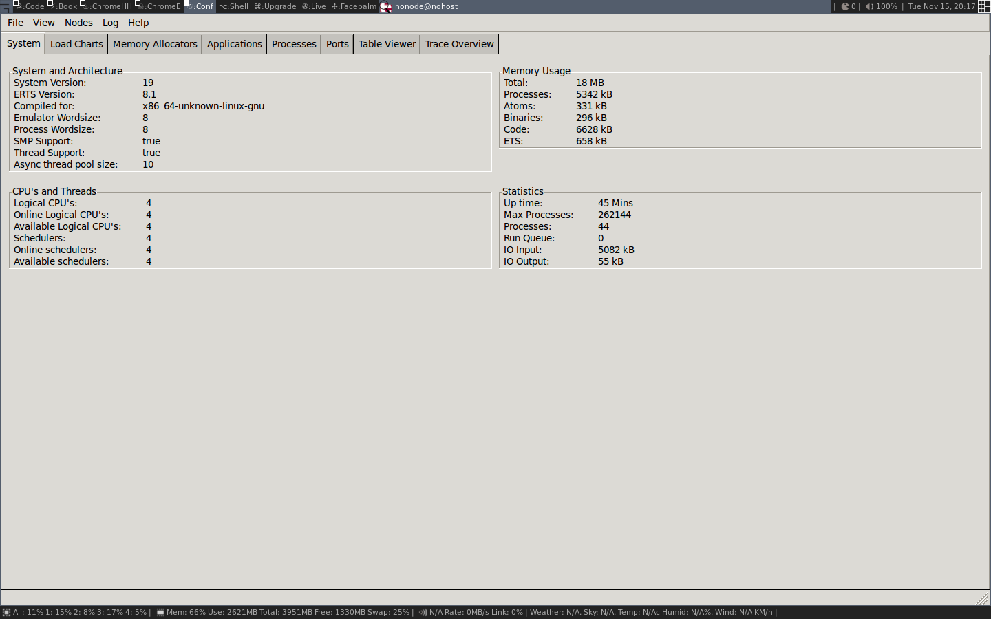
我们将在本章和下一章中详细讨论这些信息。现在我们只用Observer来观察正在运行中的进程。首先我们看一下 Applications 标签,它显示了运行系统的监督树:
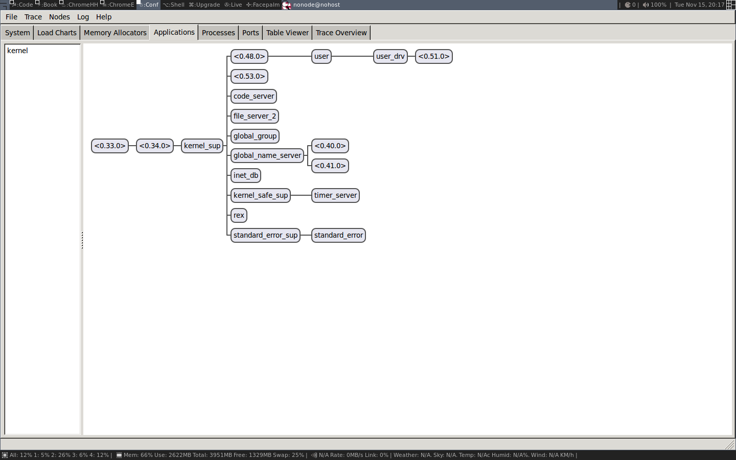
在这里,我们得到了流程如何链接的图形视图。这是一种用来了解系统被如何构建的好方法。您还会很好的感觉到,进程就像漂浮在空间中的孤立实体通过链接相互连接。
为了得到一些关于进程的有用信息,我们切换到 Processes 选项卡:
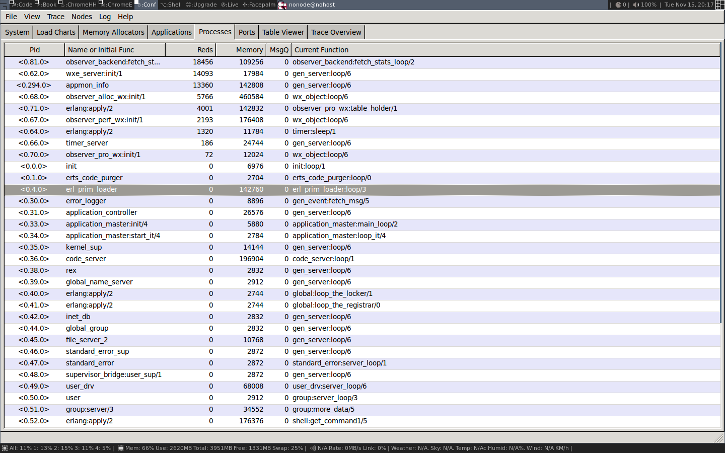
在这个视图中,我们得到了与 shell 中的 i/0 基本相同的信息。我们可以看到 pid、注册名称、规约值数量、内存使用量、消息数量和当前函数。
我们也可以通过双击某行的行来查看进程(例如 code server),以获得通过 process_info/2 可以获得的信息:
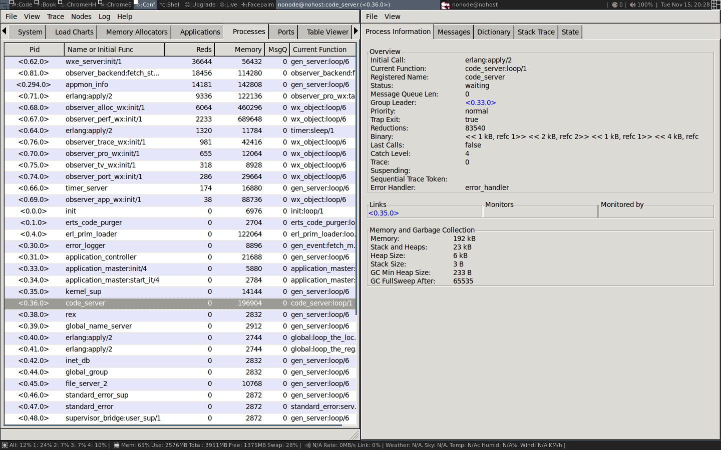
我们现在不讨论所有这些信息的意义,但如果你继续阅读,所有的信息最终都会被揭示。
既然我们已经基本了解了什么是进程,以及一些用于查找和检查系统中进程的工具,那么我们就可以深入了解进程是如何实现的了。
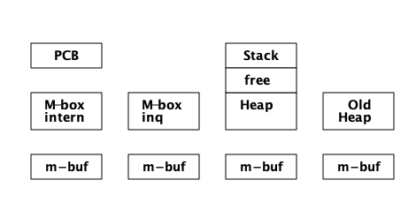
3.2. 进程就是内存
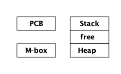
一个进程基本上是四个内存块:一个_stack_,一个_heap_,一个_message区域,和一个进程控制块_ (PCB)。
栈用于通过存储返回地址来跟踪程序执行情况、向函数传递参数,以及保存本地变量。更大的结构,如列表和元组被存储在堆中。
Message area,也称为信箱 ( mailbox ) ,用于存储从其他进程发送给自身进程的消息。进程控制块用于跟踪进程的状态。
如图,以内存视角查看进程:
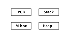
这幅关于进程的图已经非常简化,我们将对更精细的版本进行多次迭代,以得到更精确的图。
栈、堆和邮箱内存都是动态分配的,可以根据需要扩容或缩容。我们将在后面的章节中看到它是如何工作的。另一方面,PCB 是静态分配的,并且包含许多控制进程的字段。
实际上,我们可以通过使用 HiPE’s Built In Functions (HiPE BIFs) 中的自省来检查其中一些内存区域。有了这些 BIFs,我们可以打印出栈、堆和 PCB 的内存中的内容。原始数据会被打印出来,在大多数情况下,人类可读的版本会与数据一起打印出来。要真正了解检查内存时我们所看到的一切,我们需要知道更多关于 Erlang 标签方案 (将在 Chapter 4 中介绍)、执行模型和错误处理(将在 Chapter 5 中介绍),但是使用这些工具将给我们一个很好的视图来说明,进程其实就是内存。
使用 hipe_bifs:show_estack/1 我们可以看到进程栈的上下文:
1> hipe_bifs:show_estack(self()).
 |                BEAM  STACK              |
 |            Address |           Contents |
 |--------------------|--------------------| BEAM ACTIVATION RECORD
 | 0x00007f9cc3238310 | 0x00007f9cc2ea6fe8 | BEAM PC shell:exprs/7 + 0x4e
 | 0x00007f9cc3238318 | 0xfffffffffffffffb | []
 | 0x00007f9cc3238320 | 0x000000000000644b | none
 |--------------------|--------------------| BEAM ACTIVATION RECORD
 | 0x00007f9cc3238328 | 0x00007f9cc2ea6708 | BEAM PC shell:eval_exprs/7 + 0xf
 | 0x00007f9cc3238330 | 0xfffffffffffffffb | []
 | 0x00007f9cc3238338 | 0xfffffffffffffffb | []
 | 0x00007f9cc3238340 | 0x000000000004f3cb | cmd
 | 0x00007f9cc3238348 | 0xfffffffffffffffb | []
 | 0x00007f9cc3238350 | 0x00007f9cc3237102 | {value,#Fun<shell.5.104321512>}
 | 0x00007f9cc3238358 | 0x00007f9cc323711a | {eval,#Fun<shell.21.104321512>}
 | 0x00007f9cc3238360 | 0x00000000000200ff | 8207
 | 0x00007f9cc3238368 | 0xfffffffffffffffb | []
 | 0x00007f9cc3238370 | 0xfffffffffffffffb | []
 | 0x00007f9cc3238378 | 0xfffffffffffffffb | []
 |--------------------|--------------------| BEAM ACTIVATION RECORD
 | 0x00007f9cc3238380 | 0x00007f9cc2ea6300 | BEAM PC shell:eval_loop/3 + 0x47
 | 0x00007f9cc3238388 | 0xfffffffffffffffb | []
 | 0x00007f9cc3238390 | 0xfffffffffffffffb | []
 | 0x00007f9cc3238398 | 0xfffffffffffffffb | []
 | 0x00007f9cc32383a0 | 0xfffffffffffffffb | []
 | 0x00007f9cc32383a8 | 0x000001a000000343 | <0.52.0>
 |....................|....................| BEAM CATCH FRAME
 | 0x00007f9cc32383b0 | 0x0000000000005a9b | CATCH 0x00007f9cc2ea67d8
 |                    |                    |  (BEAM shell:eval_exprs/7 + 0x29)
 |********************|********************|
 |--------------------|--------------------| BEAM ACTIVATION RECORD
 | 0x00007f9cc32383b8 | 0x000000000093aeb8 | BEAM PC normal-process-exit
 | 0x00007f9cc32383c0 | 0x00000000000200ff | 8207
 | 0x00007f9cc32383c8 | 0x000001a000000343 | <0.52.0>
 |--------------------|--------------------|
true
2>
我们将 Chapter 4 中进一步研究的栈和堆中的值。堆的内容由 hipe_bifs:show_heap/1 打印。我们不想在这里列出一个大的堆,所以我们将生成一个不做任何事情的新进程并显示它的堆:
2> hipe_bifs:show_heap(spawn(fun () -> ok end)).
From: 0x00007f7f33ec9588 to 0x00007f7f33ec9848
 |                 H E A P                 |
 |            Address |           Contents |
 |--------------------|--------------------|
 | 0x00007f7f33ec9588 | 0x00007f7f33ec959a | #Fun<erl_eval.20.52032458>
 | 0x00007f7f33ec9590 | 0x00007f7f33ec9839 | [[]]
 | 0x00007f7f33ec9598 | 0x0000000000000154 | Thing Arity(5) Tag(20)
 | 0x00007f7f33ec95a0 | 0x00007f7f3d3833d0 | THING
 | 0x00007f7f33ec95a8 | 0x0000000000000000 | THING
 | 0x00007f7f33ec95b0 | 0x0000000000600324 | THING
 | 0x00007f7f33ec95b8 | 0x0000000000000000 | THING
 | 0x00007f7f33ec95c0 | 0x0000000000000001 | THING
 | 0x00007f7f33ec95c8 | 0x000001d0000003a3 | <0.58.0>
 | 0x00007f7f33ec95d0 | 0x00007f7f33ec95da | {[],{eval...
 | 0x00007f7f33ec95d8 | 0x0000000000000100 | Arity(4)
 | 0x00007f7f33ec95e0 | 0xfffffffffffffffb | []
 | 0x00007f7f33ec95e8 | 0x00007f7f33ec9602 | {eval,#Fun<shell.21.104321512>}
 | 0x00007f7f33ec95f0 | 0x00007f7f33ec961a | {value,#Fun<shell.5.104321512>}...
 | 0x00007f7f33ec95f8 | 0x00007f7f33ec9631 | [{clause...

 ...

 | 0x00007f7f33ec97d0 | 0x00007f7f33ec97fa | #Fun<shell.5.104321512>
 | 0x00007f7f33ec97d8 | 0x00000000000000c0 | Arity(3)
 | 0x00007f7f33ec97e0 | 0x0000000000000e4b | atom
 | 0x00007f7f33ec97e8 | 0x000000000000001f | 1
 | 0x00007f7f33ec97f0 | 0x0000000000006d0b | ok
 | 0x00007f7f33ec97f8 | 0x0000000000000154 | Thing Arity(5) Tag(20)
 | 0x00007f7f33ec9800 | 0x00007f7f33bde0c8 | THING
 | 0x00007f7f33ec9808 | 0x00007f7f33ec9780 | THING
 | 0x00007f7f33ec9810 | 0x000000000060030c | THING
 | 0x00007f7f33ec9818 | 0x0000000000000002 | THING
 | 0x00007f7f33ec9820 | 0x0000000000000001 | THING
 | 0x00007f7f33ec9828 | 0x000001d0000003a3 | <0.58.0>
 | 0x00007f7f33ec9830 | 0x000001a000000343 | <0.52.0>
 | 0x00007f7f33ec9838 | 0xfffffffffffffffb | []
 | 0x00007f7f33ec9840 | 0xfffffffffffffffb | []
 |--------------------|--------------------|
true
3>
我们也可以通过 hipe_bifs:show_pcb/1 来打印 PCB 中的字段:
3> hipe_bifs:show_pcb(self()).
 P: 0x00007f7f3cbc0400
 ---------------------------------------------------------------
 Offset| Name        | Value              | *Value             |
     0 | id          | 0x000001d0000003a3 |                    |
    72 | htop        | 0x00007f7f33f15298 |                    |
    96 | hend        | 0x00007f7f33f16540 |                    |
    88 | heap        | 0x00007f7f33f11470 |                    |
   104 | heap_sz     | 0x0000000000000a1a |                    |
    80 | stop        | 0x00007f7f33f16480 |                    |
   592 | gen_gcs     | 0x0000000000000012 |                    |
   594 | max_gen_gcs | 0x000000000000ffff |                    |
   552 | high_water  | 0x00007f7f33f11c50 |                    |
   560 | old_hend    | 0x00007f7f33e90648 |                    |
   568 | old_htop    | 0x00007f7f33e8f8e8 |                    |
   576 | old_head    | 0x00007f7f33e8e770 |                    |
   112 | min_heap_.. | 0x00000000000000e9 |                    |
   328 | rcount      | 0x0000000000000000 |                    |
   336 | reds        | 0x0000000000002270 |                    |
    16 | tracer      | 0xfffffffffffffffb |                    |
    24 | trace_fla.. | 0x0000000000000000 |                    |
   344 | group_lea.. | 0x0000019800000333 |                    |
   352 | flags       | 0x0000000000002000 |                    |
   360 | fvalue      | 0xfffffffffffffffb |                    |
   368 | freason     | 0x0000000000000000 |                    |
   320 | fcalls      | 0x00000000000005a2 |                    |
   384 | next        | 0x0000000000000000 |                    |
    48 | reg         | 0x0000000000000000 |                    |
    56 | nlinks      | 0x00007f7f3cbc0750 |                    |
   616 | mbuf        | 0x0000000000000000 |                    |
   640 | mbuf_sz     | 0x0000000000000000 |                    |
   464 | dictionary  | 0x0000000000000000 |                    |
   472 | seq..clock  | 0x0000000000000000 |                    |
   480 | seq..astcnt | 0x0000000000000000 |                    |
   488 | seq..token  | 0xfffffffffffffffb |                    |
   496 | intial[0]   | 0x000000000000320b |                    |
   504 | intial[1]   | 0x0000000000000c8b |                    |
   512 | intial[2]   | 0x0000000000000002 |                    |
   520 | current     | 0x00007f7f3be87c20 | 0x000000000000ed8b |
   296 | cp          | 0x00007f7f3d3a5100 | 0x0000000000440848 |
   304 | i           | 0x00007f7f3be87c38 | 0x000000000044353a |
   312 | catches     | 0x0000000000000001 |                    |
   224 | arity       | 0x0000000000000000 |                    |
   232 | arg_reg     | 0x00007f7f3cbc04f8 | 0x000000000000320b |
   240 | max_arg_reg | 0x0000000000000006 |                    |
   248 | def..reg[0] | 0x000000000000320b |                    |
   256 | def..reg[1] | 0x0000000000000c8b |                    |
   264 | def..reg[2] | 0x00007f7f33ec9589 |                    |
   272 | def..reg[3] | 0x0000000000000000 |                    |
   280 | def..reg[4] | 0x0000000000000000 |                    |
   288 | def..reg[5] | 0x00000000000007d0 |                    |
   136 | nsp         | 0x0000000000000000 |                    |
   144 | nstack      | 0x0000000000000000 |                    |
   152 | nstend      | 0x0000000000000000 |                    |
   160 | ncallee     | 0x0000000000000000 |                    |
    56 | ncsp        | 0x0000000000000000 |                    |
    64 | narity      | 0x0000000000000000 |                    |
 ---------------------------------------------------------------

true
4>
现在有了这些检查工具的支持,我们准备看看这些领域的PCB意味着什么。
3.3. 进程控制块(PCB)
进程控制块包含控制进程行为和当前状态的所有字段。在本节和本章的其余部分,我们将介绍最重要的字段。我们将在本章中省略与执行和跟踪有关的一些字段,而在 Chapter 5 中讨论那些字段。
如果你想比我们在本章中介绍的内容了解的更深入,你可以看看PCB 的 C 源代码。PCB在文件 link: ' erl_process.h ' 中被实现为一个名为 process 的 C 结构体。
`id` 包含进程的 ID (或 PID)。
0 | id | 0x000001d0000003a3 | |
进程 ID 是一个 Erlang 项式,因此会有 tag (参见 Chapter 4 )。这意味着4个最低有效位是一个标签 (tag, 0011)。在代码部分,有一个检查 Erlang 项式的模块(请参阅 show.erl ),我们将在关于类型的一章中介绍它。不过,我们现在可以使用它来检查加了标签的项式的类型。
4> show:tag_to_type(16#0000001d0000003a3).
pid
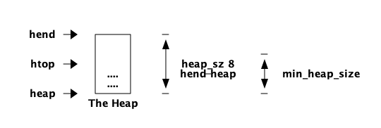
5>字段 htop 和 stop 分别是指向堆和栈顶部的指针,也就是说,它们指向堆或栈的下一个空闲槽。字段 heap (start) 和 hend 指向整个堆的开始和结束, heap_sz 用单词表示堆的大小。在64位机器上 hend - heap = heap_sz * 8 ,在32位机器上 hend - heap = heap_sz * 4 。
字段 min_heap_size 是堆开始时的大小,它不会缩小到小于这个值,默认值是 233。
我们现在可以用 PCB 控制堆的形状的字段来精炼进程堆的图片:
但是,等一下,为什么我们有堆开始和堆结束,但没有栈的开始和结束呢?这是因为 BEAM 使用了一种通过同时分配堆和堆栈来节省空间和指针的技巧。现在,我们第一次修正脑海里进程的内存图像。堆和栈实际上在同一个内存区域:
栈向低内存地址增长,堆向高内存地址增长,所以我们也可以通过添加栈顶指针来优化堆的图片:
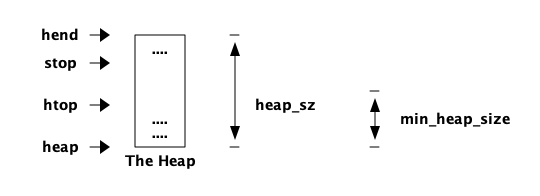
当指针 htop 和 stop 相遇,进程将耗尽空闲内存,必须进行垃圾收集来释放内存。
3.4. 垃圾收集器 (GC)
Erlang 使用每个进程复制分代垃圾收集器来管理堆内存。当堆 (或栈,因为它们共享分配的内存块) 上没有更多空间时,垃圾收集器就会开始释放内存。
GC 分配一个名为 to space 的新内存区域。然后,它遍历栈以找到所有活动根,并跟踪每个根,将堆上的数据复制到新堆。最后,它还将栈复制到新堆并释放旧的内存区域。
GC 是由 PCB 中的以下字段控制的:
    Eterm *high_water;
    Eterm *old_hend;    /* Heap pointers for generational GC. */
    Eterm *old_htop;
    Eterm *old_heap;
    Uint max_heap_size; /* Maximum size of heap (in words). */
    Uint16 gen_gcs;	/* Number of (minor) generational GCs. */
    Uint16 max_gen_gcs;	/* Max minor gen GCs before fullsweep. */
由于垃圾收集器是分代的,所以大多数时候它将使用启发式方法来查看新数据。也就是说,在所谓的 minor collection 中,GC 只查看栈的顶部并将新数据移动到新堆中。旧数据,即在堆上的 high_water 标记 (见下图) 以下分配的数据,被移动到一个称为旧堆(old heap)的特殊区域。
大多数时候,每个进程都有另一个堆区域:旧堆,由PCB中的字段 old_heap、 old_htop 以及 old_hend 处理。这几乎把我们带回了原来的进程图,即四个内存区域:
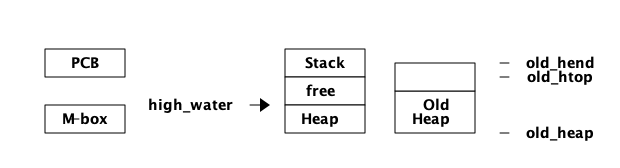
当一个进程启动时是没有旧堆的,但是一旦年轻数据成熟为旧数据,并且存在垃圾收集,就会分配旧堆。当有 major collection (也称为 full sweep) 时,旧堆被垃圾收集。请参阅 Chapter 12 了解垃圾收集如何工作的更多细节。在那一章中,我们还将看到如何跟踪和修复与内存相关的问题。
3.5. 信箱(Mailbox)和消息传递
进程通信通过消息传递完成。进程发送被实现,以便发送进程将消息从自己的堆复制到接收进程的邮箱。
在 Erlang 的 早期,并发是通过调度器中的多任务来实现的。我们将在本章后面的调度器一节中更多地讨论并发性,现在值得注意的是,在 Erlang 的第一版中没有并行性,那时一次只能同时运行一个进程。在那个版本中,发送进程可以直接在接收进程的堆上写入数据。
3.5.1. 并行发送消息
当多核系统被引入,Erlang 实现被扩展为多个调度器来调度多个并行运行的进程时,在不获取接收方的 main lock 的情况下直接写另一个进程的堆就不再安全了。此时引入了 m-bufs 的概念 (也称为“堆片段”, heap fragments)。 m-bufs 是一个在进程堆外的内存区域,其他进程可以安全地写入数据。
如果发送进程不能获得锁,它就可以将消息写入 m-buf 。当消息的所有数据都已复制到 m-buf 时,该消息将通过邮箱链接到进程。链接(LINK_MESSAGE, erl_message.h)将消息追加到接收方的消息队列最后。
垃圾收集器然后将这些消息复制到进程的堆中。为了减少 GC 时的压力,邮箱被分成两个列表,一个包含已看到的消息,另一个包含新消息。GC 不必查看任何新消息,因为我们知道它们将在 GC 中存活下来(它们仍然在邮箱中),这样我们可以避免一些复制。
3.6. 无锁消息传递
在 Erlang 19 中引入了一个新的可以每个进程分别设置的 message_queue_data ,它可以取 on_heap 或 off_heap 的值。当设置为 on_heap 时,发送进程将首先尝试获取接收方的 main lock ,如果成功,则消息将直接复制到接收方的堆上。以上场景只有在接收方被挂起并且没有其他进程获取该锁以发送给同一进程时才发生。如果发送方不能获得锁,它将分配一个堆片段并将消息复制到那里。
如果标志设置为 off_heap ,发送方将不会尝试获得锁,而是直接写入堆片段。这将减少锁争用,但是分配一个堆片段比直接写入已经分配的进程堆的开销更大,而且会导致更大的内存使用。可能进程已经分配了一个大的空堆,但发送者依然会将新消息写入新的堆片段。
使用 on_heap 方式,所有消息,包括直接分配在堆上的消息和堆碎片中的消息,都是被 GC 复制的。如果消息队列很大,许多消息没有处理,因此仍然是活动的,它们将被提升到旧堆,进程堆的大小将增加,从而导致更高的内存使用量。
当消息被复制到接收进程时,所有消息都被添加到一个链表 ( mailbox ) 中。如果消息被复制到接收进程的堆中,该消息将链接到 “内部消息队列” ( internal message queue ,或 seen 消息) 并由 GC 检查。在 off_heap 分配方案中,新消息被放置在 “外部” ( external ) message in queue 中,并被 GC 忽略。
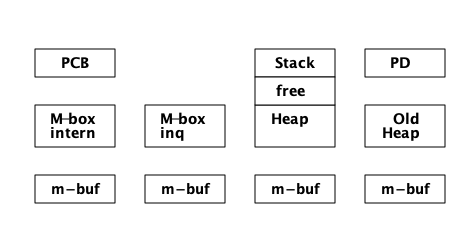
3.6.1. 消息的内存区域
现在,我们可以再次将进程描述为四个内存区域的看法组一个修正了。现在每个进程由五个内存区域 ( heap ,stack, PCB , internal mailbox, 和 external mailbox ) 和不同数量的堆碎片 ( m-bufs )组成:
每个邮箱都包含长度和两个指针信息, internal queue 的信息存储在字段 msg.len, msg.first, msg.last 中。用于内部队列和msg_inq,external in queue 的信息存储在 msg_inq.len, msg_inq.first, 以及 msg_inq.last 中。还有一个指针指向下一个要查看的消息( msg.save ),以实现选择性接收。
3.6.2. 检查消息处理
让我们使用自省工具来更详细地了解它是如何工作的。我们首先在邮箱中设置一个带有消息的进程,然后查看PCB。
4> P = spawn(fun() -> receive stop -> ok end end).
<0.63.0>
5> P ! start.
start
6> hipe_bifs:show_pcb(P).

...
  408 | msg.first     | 0x00007fd40962d880 |                    |
  416 | msg.last      | 0x00007fd40962d880 |                    |
  424 | msg.save      | 0x00007fd40962d880 |                    |
  432 | msg.len       | 0x0000000000000001 |                    |
  696 | msg_inq.first | 0x0000000000000000 |                    |
  704 | msg_inq.last  | 0x00007fd40a306238 |                    |
  712 | msg_inq.len   | 0x0000000000000000 |                    |
  616 | mbuf          | 0x0000000000000000 |                    |
  640 | mbuf_sz       | 0x0000000000000000 |                    |
...
从这里我们可以看到消息队列中有一条消息, first, last 和 save 指针都指向该消息。
如前所述,可以通过设置标志 message_queue_data 来强制消息进入 in queue 队列。我们可以用以下程序来尝试:
-module(msg).

-export([send_on_heap/0
        ,send_off_heap/0]).

send_on_heap() -> send(on_heap).
send_off_heap() -> send(off_heap).

send(How) ->
  %% Spawn a function that loops for a while
  P2 = spawn(fun () -> receiver(How) end),
  %% spawn a sending process
  P1 = spawn(fun () -> sender(P2) end),
  P1.

sender(P2) ->
  %% Send a message that ends up on the heap
  %%  {_,S} = erlang:process_info(P2, heap_size),
  M = loop(0),
  P2 ! self(),
  receive ready -> ok end,
  P2 ! M,
  %% Print the PCB of P2
  hipe_bifs:show_pcb(P2),
  ok.

receiver(How) ->
  erlang:process_flag(message_queue_data,How),
  receive P -> P ! ready end,
  %%  loop(100000),
  receive x -> ok end,
  P.


loop(0) -> [done];
loop(N) -> [loop(N-1)].
有了这个程序,我们可以试着使用 on_heap 或 off_heap 模式发送消息,并在每次发送后查看 PCB。使用 on_heap 模式,我们得到了与之前的消息发送相同的结果:
5> msg:send_on_heap().

...

  408 | msg.first     | 0x00007fd4096283c0 |                    |
  416 | msg.last      | 0x00007fd4096283c0 |                    |
  424 | msg.save      | 0x00007fd40a3c1048 |                    |
  432 | msg.len       | 0x0000000000000001 |                    |
  696 | msg_inq.first | 0x0000000000000000 |                    |
  704 | msg_inq.last  | 0x00007fd40a3c1168 |                    |
  712 | msg_inq.len   | 0x0000000000000000 |                    |
  616 | mbuf          | 0x0000000000000000 |                    |
  640 | mbuf_sz       | 0x0000000000000000 |                    |

...
如果我们尝试发送到一个设置为 off_heap 标志的进程,消息会落在 in queue 队列中:
6> msg:send_off_heap().

...

  408 | msg.first     | 0x0000000000000000 |                    |
  416 | msg.last      | 0x00007fd40a3c0618 |                    |
  424 | msg.save      | 0x00007fd40a3c0618 |                    |
  432 | msg.len       | 0x0000000000000000 |                    |
  696 | msg_inq.first | 0x00007fd3b19f1830 |                    |
  704 | msg_inq.last  | 0x00007fd3b19f1830 |                    |
  712 | msg_inq.len   | 0x0000000000000001 |                    |
  616 | mbuf          | 0x0000000000000000 |                    |
  640 | mbuf_sz       | 0x0000000000000000 |                    |

...
3.6.3. 向进程发送消息的过程
现在我们将忽略分布情况,也就是说我们不会考虑Erlang节点之间发送的消息。想象两个过程 P1 和 P2。进程 P1 想向进程 `P2`发送一条消息(Msg),如图所示:
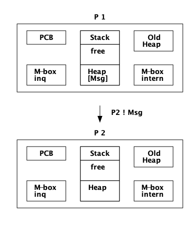
进程 P1 将执行以下步骤:
-
计算 Msg 的大小。
-
为消息分配空间(如前所述,在
P2的堆上或堆外)。 -
将 Msg 从
P1的堆复制到分配的空间。 -
分配并填充一个 ErlMessage 结构体来包装消息。
-
将 ErlMessage 链接到 ErlMsgQueue 或 ErlMsgInQueue。
如果进程 P2 被挂起,没有其他进程尝试向 P2 发送消息,并且堆上有空间,分配策略为 on_heap,那么消息将直接在堆上写入:
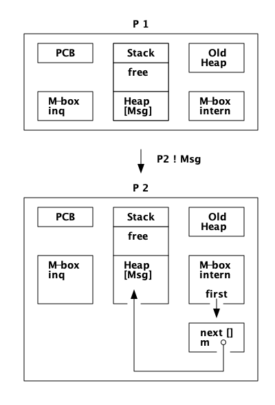
如果 P1 不能获得 P2 的 main lock,或者 P2 的堆空间不够,分配策略为 on_heap,那么消息将写入 m-buf,但链接到内部邮箱:
在一次GC之后,消息将被移动到堆中。
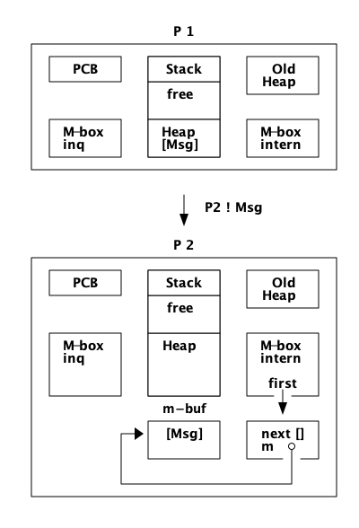
如果分配策略是 off_heap,消息将以 m-buf 结束,并链接到外部邮箱:
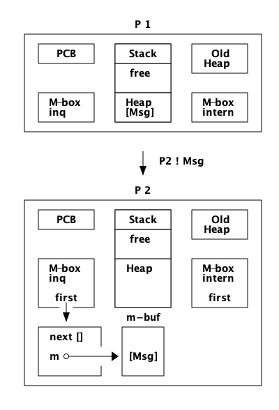
在一次 GC 之后,消息仍然在 m-buf 中。直到接收到该消息并从堆上的其他对象或从栈可访问该消息,该消息才会在 GC 期间被复制到进程堆中。
3.6.4. 消息接收
Erlang 支持选择性接收,这意味着不匹配的消息可以留在邮箱中等待以后收取。如果消息不匹配,即使信箱中有消息的时候,进程也可能是挂起的。 msg.save 字段包含一个指向下一条要查看的消息的指针。
在后面的章节中,我们将详细介绍 m-bufs 以及垃圾收集器如何处理邮箱。在后面的章节中,我们还将详细介绍如何在 BEAM 中实现消息接收。
3.6.5. 消息传递调优
使用 Erlang 19 中引入的新 message_queue_data 标志,您可以以一种新的方式用内存空间来 ”交换“ 执行时间。如果接收进程已经过载并一直持有 main lock,那么使用 off_heap 分配可能是一个好策略,这种策略能让发送进程快速地将消息转储到 m-buf 中。
如果两个进程有一个良好平衡的生产者消费者行为,其中没有真正争夺进程锁,那么直接在接收者堆上分配会更快,并且会使用更少的内存。
如果接收方已经过载,且不断接受消息,处理消息的速度慢与接受新消息的速度,那么它实际上可能会开始使用更多的内存,因为消息被不断复制到堆中,并迁移到旧堆中。由于未读消息被认为是活动的,因此堆将不断增长并使用更多内存。
为了找出哪种分配策略最适合你的系统,你需要对它进行基准测试和行为度量。要做的第一个也是最简单的测试可能是在系统开始时更改默认的分配策略。ERTS 的 hmqd 标志将默认策略设置为 off_heap 或 on_heap。如果启动Erlang 时没有更改此标志,则默认为 on_heap。通过设置基准,让 Erlang 以 +hmqd off_heap 方式启动,您可以测试如果所有进程都使用非堆分配,系统的表现是更好还是更差。然后,您可能希望找到瓶颈进程,并通过配置切换分配策略来只测试这些进程。
3.7. 进程字典(PD)
实际上,进程中还有一个可以存储 Erlang 项式的内存区域,即 Process Dictionary。
Process Dictionary (PD) 是一个进程的本地键值存储。这样做的一个优点是,所有的键和值都存储在堆中,不需要像 send 或 ETS 表那样进行复制。
我们现在可以用另一个内存区域 - PD,进程字典,来更新我们对进程观点:
对于 PD 这么小的数组,在长度增长之前,你肯定会遇到一些碰撞。每个哈希值指向一个具有键值对的 bucket。bucket 实际上是堆上的 Erlang list。list 中的每个条目都是同样存储在堆中的二元元组({key, Value})。
在PD中放置一个元素并不是完全自由的,它会导致一个额外的元组和一个缺点,并可能导致垃圾收集被触发。更新位于 bucket 中的 dictionary 中的 key,会导致整个bucket (整个列表) 被重新分配,以确保我们不会获得从旧堆指向新堆的指针。(在 Chapter 12 中,我们将看到垃圾收集如何工作的细节。)
3.8. 深入
在本章中,我们已经了解了流程是如何实现的。特别地,我们查看了进程的内存是如何组织的,消息是如何传递的,以及PCB中的信息。我们还介绍了一些用于检查进程自检的工具,如 erlang:process_info 和 hipe:show*_bifs。
使用函数 erlang:processes/0 和 erlang:process_info/1,2 检查系统中的进程。以下是一些可以尝试的功能:
1> Ps = erlang:processes().
[<0.0.0>,<0.3.0>,<0.6.0>,<0.7.0>,<0.9.0>,<0.10.0>,<0.11.0>,
 <0.12.0>,<0.13.0>,<0.14.0>,<0.15.0>,<0.16.0>,<0.17.0>,
 <0.19.0>,<0.20.0>,<0.21.0>,<0.22.0>,<0.23.0>,<0.24.0>,
 <0.25.0>,<0.26.0>,<0.27.0>,<0.28.0>,<0.29.0>,<0.33.0>]
2> P = self().
<0.33.0>
3> erlang:process_info(P).
[{current_function,{erl_eval,do_apply,6}},
 {initial_call,{erlang,apply,2}},
 {status,running},
 {message_queue_len,0},
 {messages,[]},
 {links,[<0.27.0>]},
 {dictionary,[]},
 {trap_exit,false},
 {error_handler,error_handler},
 {priority,normal},
 {group_leader,<0.26.0>},
 {total_heap_size,17730},
 {heap_size,6772},
 {stack_size,24},
 {reductions,25944},
 {garbage_collection,[{min_bin_vheap_size,46422},
                      {min_heap_size,233},
                      {fullsweep_after,65535},
                      {minor_gcs,1}]},
 {suspending,[]}]
 4>  lists:keysort(2,[{P,element(2,erlang:process_info(P,
     total_heap_size))} || P <- Ps]).
[{<0.10.0>,233},
 {<0.13.0>,233},
 {<0.14.0>,233},
 {<0.15.0>,233},
 {<0.16.0>,233},
 {<0.17.0>,233},
 {<0.19.0>,233},
 {<0.20.0>,233},
 {<0.21.0>,233},
 {<0.22.0>,233},
 {<0.23.0>,233},
 {<0.25.0>,233},
 {<0.28.0>,233},
 {<0.29.0>,233},
 {<0.6.0>,752},
 {<0.9.0>,752},
 {<0.11.0>,1363},
 {<0.7.0>,1597},
 {<0.0.0>,1974},
 {<0.24.0>,2585},
 {<0.26.0>,6771},
 {<0.12.0>,13544},
 {<0.33.0>,13544},
 {<0.3.0>,15143},
 {<0.27.0>,32875}]
9>
4. Erlang 类型系统和标签
要理解 ERTS 最重要的方面之一,是 ERTS 如何存储数据,即 Erlang 项式如何存储在内存中。这为你理解垃圾收集如何工作、消息传递如何工作提供了基础,并使你了解需要多少内存。
在本章中,您将学习Erlang 的基本数据类型以及如何在ERTS中实现它们。这些知识对于理解内存分配和垃圾收集这一章非常重要,请参阅Chapter 12。
4.1. Erlang 类型系统
Erlang 是强类型( strong typed )语言。也就是说,无法将一种类型强制转换 ( coerce ) 为另一种类型,只能从一种类型转换 ( convert ) 为另一种类型。与 C语言 比较,在 C 语言中,你可以强制一个 char 转换为一个 int,或任何类型的指针指向 ( void * )。
Erlang 类型格( lattice )是非常扁平的,只有很少的子类型,number有 整数( integer ) 和浮点( float )子类型,list有 nil(空表) 和 cons(列表单元,译注:源自list constructor) 子类型 (也可以认为每个大小的元组都有一个子类型)。
Erlang类型格
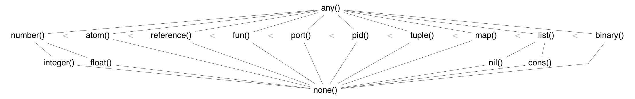
Erlang 中的所有项都有一个部分顺序 ( < 和 > ),上面型格图中各种类型在是从左到右排序的。
顺序是部分的而不是全部的,因为整数和浮点数在比较之前是要进行转换的。(1 < 1.0) 和 (1.0 < 1) 都是 false,(1 =< 1.0和1 >= 1.0) 和 (1 =/= 1.0) 都是 false。精度较低的数字被转换为精度较高的数字。通常整数被转换为浮点数。对于非常大或非常小的浮点数,如果所有有效数字都在小数点的左边,浮点数就会被转换为整数。
从 Erlang 18 开始,当比较两个 Map 的顺序时,它们的比较如下:如果一个 Map 的元素少于另一个,则认为它更小。否则,按项顺序比较键,即认为所有整数都比所有浮点数小。如果所有的键都是相同的,那么每个值对 (按键的顺序) 将进行算术比较,即首先将它们转换为相同的精度。
当比较相等时也是如此,因此 #{1 => 1.0}== #{1 => 1},但是 #{1.0 => 1}/= #{1 => 1}。
在 Erlang 18 之前的版本,key 的比较也是算术比较。
Erlang 是动态类型的。也就是说,将在运行时检查类型,如果发生类型错误,则抛出异常。编译器不会在编译时检查类型,这与 C 或 Java 等静态类型语言不同,在这些语言中,编译时可能会出现类型错误。
Erlang 类型系统的这些方面是强动态类型,类型上有一个顺序,这给语言的实现带来了一些约束。为了能够在运行时检查和比较类型,每个 Erlang 项式都必须携带它的类型。
这可以通过标记这些项式来解决。
4.2. 标签方案
在 Erlang 项式的内存表示中,为类型标记保留一些位。出于性能原因,项式被分为即时 ( immediates ) 和装箱 ( boxed ) 项式。即时项式可以放入一个机器字中,也就是说,它可以放在寄存器(译注:指通用寄存器)或堆栈槽中。装箱项式由两部分组成:标记的指针和存储在进程堆上的若干字长。除列表外,存储在堆中的装箱 ( box ) 项式都有一个头 header 和一个体 body。
目前ERTS使用分级标签方案,HiPE小组的技术报告解释了该方案背后的历史和原因。(参见 http://www.it.uu.se/research/publications/2000029/) 标签方案的实现见 erl_term.h。
基本思想是使用标签的最低有效位。由于大多数现代CPU体系结构对32位或64位的字长进行对齐,因此至少有两位是指针“未使用的”。这些位可以用作标签。不幸的是,对于 Erlang 中的所有类型,这两个位是不够的,因此需要使用更多的位。(译注:要了解这部分的内容,最好结合 OTP 源码:erl_term.h L: 70 开始阅读 )
4.2.1. 即时类型的标签
主标签(最低 2 位)被以如下方式使用:
  00 Header (on heap) CP (on stack)
  01 List (cons,译注:列表项)
  10 Boxed
  11 Immediate
(译注:以下内容源自 OTP erl_term.h, L:70)
#define _TAG_PRIMARY_SIZE   2
#define _TAG_PRIMARY_MASK  0x3
#define TAG_PRIMARY_HEADER 0x0
#define TAG_PRIMARY_LIST   0x1
#define TAG_PRIMARY_BOXED  0x2
#define TAG_PRIMARY_IMMED1 0x3
Header 标记仅用于堆上的项式标签头,稍后将对此进行详细说明。栈上的 00 表示返回地址。列表标记用于 cons 单元格,装箱类型标记用于指向堆的所有其他装箱类型的指针。即时类型标签被进一步划分如下:
 00 11 Pid
 01 11 Port
 10 11 Immediate 2
 11 11 Small integer
(译注:以下内容源自 OTP erl_term.h, L:79)
#define _TAG_IMMED1_SIZE	4
#define _TAG_IMMED1_MASK	0xF
#define _TAG_IMMED1_PID		((0x0 << _TAG_PRIMARY_SIZE) | TAG_PRIMARY_IMMED1)
#define _TAG_IMMED1_PORT	((0x1 << _TAG_PRIMARY_SIZE) | TAG_PRIMARY_IMMED1)
#define _TAG_IMMED1_IMMED2	((0x2 << _TAG_PRIMARY_SIZE) | TAG_PRIMARY_IMMED1)
#define _TAG_IMMED1_SMALL	((0x3 << _TAG_PRIMARY_SIZE) | TAG_PRIMARY_IMMED1)
Pid 和 port 是即时类型的,可以比较有效的比较大小。它们实际上只是引用,pid 是一个进程标识符,它指向一个进程。该进程不驻留在任何进程的堆中,而是由PCB处理。port 的工作方式也大致相同。
在 ERTS 中有两种类型的整数:小整数和大整数。小整数使用一个机器字减去四个标签位,即在 32位机和 64 位机上分别对应 28 位或 60 位。另一方面,大整数可以根据需要大小扩展 ( 仅受堆空间大小的限制 ),并作为装箱对象存储在堆中。
小整数的所有 4 个标记位为 1,仿真器可以在进行整数运算时进行有效的测试,以查看两个参数是否都是即时类型的。 (is_both_small(x,y) 被定义为 (x & y & 1111) == 1111).
Immediate 2 的标签被进一步划分如下:
 00 10 11 Atom
 01 10 11 Catch
 10 10 11  [UNUSED]
 11 10 11 Nil
(译注:以下内容源自 OTP erl_term.h, L:86)
#define _TAG_IMMED2_SIZE	6
#define _TAG_IMMED2_MASK	0x3F
#define _TAG_IMMED2_ATOM	((0x0 << _TAG_IMMED1_SIZE) | _TAG_IMMED1_IMMED2)
#define _TAG_IMMED2_CATCH	((0x1 << _TAG_IMMED1_SIZE) | _TAG_IMMED1_IMMED2)
#define _TAG_IMMED2_NIL		((0x3 << _TAG_IMMED1_SIZE) | _TAG_IMMED1_IMMED2)
原子由(指向) atom table 表中的索引和 atom 标签组成。要比较两个 atom 即时类型变量是否相等,只要比较两个原子的即时表示就可以。
在 atom table 中,原子被存储为这样的 C 结构体:
typedef struct atom {
    IndexSlot slot;  /* MUST BE LOCATED AT TOP OF STRUCT!!! */
    int len;         /* length of atom name */
    int ord0;        /* ordinal value of first 3 bytes + 7 bits */
    byte* name;      /* name of atom */
} Atom;
由于 len 和 ord0 字段,只要两个原子不以相同的四个字母开头,它们的顺序可以高效地进行比较。
Catch 即时类型只在堆栈上使用。它包含一个间接的指针,指向代码中的接续点(continuation point),在异常发生后执行应该从接续点继续开始。在 Chapter 8 中有更多的内容。
Nil 标记用于空列表( Nil 或 [] )。机器字的其余部分都被 1 填充。
4.2.2. 装箱项式的标签
存储在堆上的 Erlang 项式使用几个机器字。列表或 cons 列表项单元只是堆上两个连续的字:头和尾(或者在 lisp 和 ERTS 代码的某些地方称为 car 和 cdr)。
Erlang 中的字符串只是表示字符的整数列表。在 Erlang OTP R14 之前的版本中,字符串被编码为 ISO-latin-1 (ISO8859-1)。自 R14 开始,字符串被编码为 Unicode 代码列表。对于 latin-1 中的字符串,它们和 Unicode 没有区别,因为latin-1是Unicode的子集。
字符串 "hello" 在内存中看起来可能是这样的:

所有其他装箱的项式的主标签都以 Header 00 开头。标头字使用 4 位标头标记和 2 位主标头标记(00),它还具有一个 arity域,用来表示装箱类型的变量使用了多少个字存储。在32位计算机上,它看起来是这样的:aaaaaaaaaaaaaaaaaaaaaatttt00。
标签如下:
 0000	ARITYVAL (Tuples)
 0001   BINARY_AGGREGATE                |
 001s	BIGNUM with sign bit            |
 0100	REF                             |
 0101	FUN                             | THINGS
 0110	FLONUM                          |
 0111   EXPORT                          |
 1000	REFC_BINARY     |               |
 1001	HEAP_BINARY     | BINARIES      |
 1010	SUB_BINARY      |               |
 1011    [UNUSED]
 1100   EXTERNAL_PID  |                 |
 1101   EXTERNAL_PORT | EXTERNAL THINGS |
 1110   EXTERNAL_REF  |                 |
 1111   MAP
(译注:以下内容源自 OTP erl_term.h, L:92)
/*
 * HEADER representation:
 *
 *	aaaaaaaaaaaaaaaaaaaaaaaaaatttt00	arity:26, tag:4
 *
 * HEADER tags:
 *
 *	0000	ARITYVAL
 *  0001    BINARY_AGGREGATE                |
 *	001x	BIGNUM with sign bit		|
 *	0100	REF				|
 *	0101	FUN				| THINGS
 *	0110	FLONUM				|
 *  0111    EXPORT                          |
 *	1000	REFC_BINARY	|		|
 *	1001	HEAP_BINARY	| BINARIES	|
 *	1010	SUB_BINARY	|		|
 *  1011    Not used; see comment below
 *  1100    EXTERNAL_PID  |                 |
 *  1101    EXTERNAL_PORT | EXTERNAL THINGS |
 *  1110    EXTERNAL_REF  |                 |
 *  1111    MAP
 *
 * COMMENTS:
 *
 * - The tag is zero for arityval and non-zero for thing headers.
 * - A single bit differentiates between positive and negative bignums.
 * - If more tags are needed, the REF and and EXTERNAL_REF tags could probably
 *   be combined to one tag.
 *
 * XXX: globally replace XXX_SUBTAG with TAG_HEADER_XXX
 */
#define ARITYVAL_SUBTAG		(0x0 << _TAG_PRIMARY_SIZE) /* TUPLE */
#define BIN_MATCHSTATE_SUBTAG	(0x1 << _TAG_PRIMARY_SIZE)
#define POS_BIG_SUBTAG		(0x2 << _TAG_PRIMARY_SIZE) /* BIG: tags 2&3 */
#define NEG_BIG_SUBTAG		(0x3 << _TAG_PRIMARY_SIZE) /* BIG: tags 2&3 */
#define _BIG_SIGN_BIT		(0x1 << _TAG_PRIMARY_SIZE)
#define REF_SUBTAG		(0x4 << _TAG_PRIMARY_SIZE) /* REF */
#define FUN_SUBTAG		(0x5 << _TAG_PRIMARY_SIZE) /* FUN */
#define FLOAT_SUBTAG		(0x6 << _TAG_PRIMARY_SIZE) /* FLOAT */
#define EXPORT_SUBTAG		(0x7 << _TAG_PRIMARY_SIZE) /* FLOAT */
#define _BINARY_XXX_MASK	(0x3 << _TAG_PRIMARY_SIZE)
#define REFC_BINARY_SUBTAG	(0x8 << _TAG_PRIMARY_SIZE) /* BINARY */
#define HEAP_BINARY_SUBTAG	(0x9 << _TAG_PRIMARY_SIZE) /* BINARY */
#define SUB_BINARY_SUBTAG	(0xA << _TAG_PRIMARY_SIZE) /* BINARY */
/*   _BINARY_XXX_MASK depends on 0xB being unused */
#define EXTERNAL_PID_SUBTAG	(0xC << _TAG_PRIMARY_SIZE) /* EXTERNAL_PID */
#define EXTERNAL_PORT_SUBTAG	(0xD << _TAG_PRIMARY_SIZE) /* EXTERNAL_PORT */
#define EXTERNAL_REF_SUBTAG	(0xE << _TAG_PRIMARY_SIZE) /* EXTERNAL_REF */
#define MAP_SUBTAG		(0xF << _TAG_PRIMARY_SIZE) /* MAP */


#define _TAG_HEADER_ARITYVAL       (TAG_PRIMARY_HEADER|ARITYVAL_SUBTAG)
#define _TAG_HEADER_FUN	           (TAG_PRIMARY_HEADER|FUN_SUBTAG)
#define _TAG_HEADER_POS_BIG        (TAG_PRIMARY_HEADER|POS_BIG_SUBTAG)
#define _TAG_HEADER_NEG_BIG        (TAG_PRIMARY_HEADER|NEG_BIG_SUBTAG)
#define _TAG_HEADER_FLOAT          (TAG_PRIMARY_HEADER|FLOAT_SUBTAG)
#define _TAG_HEADER_EXPORT         (TAG_PRIMARY_HEADER|EXPORT_SUBTAG)
#define _TAG_HEADER_REF            (TAG_PRIMARY_HEADER|REF_SUBTAG)
#define _TAG_HEADER_REFC_BIN       (TAG_PRIMARY_HEADER|REFC_BINARY_SUBTAG)
#define _TAG_HEADER_HEAP_BIN       (TAG_PRIMARY_HEADER|HEAP_BINARY_SUBTAG)
#define _TAG_HEADER_SUB_BIN        (TAG_PRIMARY_HEADER|SUB_BINARY_SUBTAG)
#define _TAG_HEADER_EXTERNAL_PID   (TAG_PRIMARY_HEADER|EXTERNAL_PID_SUBTAG)
#define _TAG_HEADER_EXTERNAL_PORT  (TAG_PRIMARY_HEADER|EXTERNAL_PORT_SUBTAG)
#define _TAG_HEADER_EXTERNAL_REF   (TAG_PRIMARY_HEADER|EXTERNAL_REF_SUBTAG)
#define _TAG_HEADER_BIN_MATCHSTATE (TAG_PRIMARY_HEADER|BIN_MATCHSTATE_SUBTAG)
#define _TAG_HEADER_MAP	           (TAG_PRIMARY_HEADER|MAP_SUBTAG)


#define _TAG_HEADER_MASK	0x3F
#define _HEADER_SUBTAG_MASK	0x3C	/* 4 bits for subtag */
#define _HEADER_ARITY_OFFS	6
只带有 arity 的 元组类型 被存储在堆中,然后用 arity 下面的字表示每个元素。空的tuple{}与单词0一样存储 ( header 标记00、tuple 标记 0000 和 arity 0)。

binary 是一个不可变的字节数组。 binary 的内部表示有四种类型。 heap binaries 和 refc binaries 这两种类型包含二进制数据。其他两种类型,sub binaries 和 match contexts ( BINARY_AGGREGATE 标签) 子二进制文件和匹配上下文(BINARY_AGGREGATE标记)是对其他两种类型之一的较小引用。
使用 64 字节或更少空间的 binary 可以作为 heap binaries 直接存储在进程堆上。对较大的 binary 来说,它们被引用计数,且有效载荷存储在进程堆之外。对有效载荷的引用存储在进程堆上一个名为 ProcBin 的对象中。
我们将在 Chapter 12 更多地讨论二进制。
如果一个整数不能装入小整数 (字长减 4 位) 空间,它将以 “bignums” (或者叫任意精度整数) 的形式存储在堆中。bignum 在内存中有一个 header,后面跟着许多编码的字。header 中 bignum 标记的符号部分 (s) 对数字的符号进行编码(对于正数,s=0,对于负数,s=1)。
引用是一个“唯一的”( "unique") 项式,通常用于标记消息,以便实现进程邮箱上的通道。引用被实现为 82 位的计数器。在调用 make_ref/0 9671406556917033397649407 次后,计数器将折返并再次以 ref 0 重新开始。在程序生命周期内,你需要一个非常快的机器来执行那么多次 make_ref 调用。重新启动该节点后 (在这种情况下,它也将再次从0开始) 所有旧的本地 refs 都会消失。如果您将 pid 发送到另一个节点,它将成为一个 external ref,见下面描述:
在32位系统上,local ref 在堆上占用 4 个 32 位字长。在 64 位系统上,ref 在堆上占用 3 个 64 位字长。
    |00000000 00000000 00000000 11010000| Arity 3 + ref tag
    |00000000 000000rr rrrrrrrr rrrrrrrr| Data0
    |rrrrrrrr rrrrrrrr rrrrrrrr rrrrrrrr| Data1
    |rrrrrrrr rrrrrrrr rrrrrrrr rrrrrrrr| Data2
引用数为: (Data2 bsl 50) + (Data1 bsl 18) + Data0.
5. Erlang 虚拟机: BEAM
BEAM (Bogumil / Björn 抽象机)是在 Erlang 运行时系统中执行代码的机器。它是一台垃圾收集,规约值计数,虚拟,非抢占式,直接线程,寄存器式机器。如果这还不能说明什么,不用担心,在接下来的部分中,我们将介绍这些单词在此上下文中的含义。
虚拟机 BEAM 位于 Erlang 节点的核心。执行 Erlang 代码的是 BEAM。也就是说,是 BEAM 执行您的应用程序代码。理解 BEAM 是如何执行代码的,对于配置和调优您的代码至关重要。
BEAM 的设计对 BEAM 的其他部分有很大的影响。用于调度的原语会影响调度器 ( Chapter 11 ),Erlang 短语的表示以及与内存的交互会影响垃圾收集器 ( Chapter 12 )。通过理解 BEAM 的基本设计,您将更容易理解这些其他组件的实现。
5.1. 工作内存: 堆栈机?并不是!
与它的前身 JAM (Joe 's Abstract Machine) 是一个堆栈机不同,BEAM 是一个基于WAM [warren] 的寄存器机器。在堆栈机器中,指令的每个操作数首先被推入工作堆栈,然后指令弹出它的参数,然后将结果推入堆栈。
堆栈机在虚拟机和编程语言实现者中非常流行,因为它们很容易为其生成代码,而且代码变得非常紧凑。编译器不需要做任何寄存器分配,并且大多数操作不需要任何参数(在指令流中)。
编译表达式 "8 + 17 * 2." 到堆栈机器可以产生如下代码:
push 8
push 17
push 2
multiply
add
compile(String) ->
    [ParseTree] = element(2,
			  erl_parse:parse_exprs(
			    element(2,
				    erl_scan:string(String)))),
    generate_code(ParseTree).

generate_code({op, _Line, '+', Arg1, Arg2}) ->
    generate_code(Arg1) ++ generate_code(Arg2) ++ [add];
generate_code({op, _Line, '*', Arg1, Arg2}) ->
    generate_code(Arg1) ++ generate_code(Arg2) ++ [multiply];
generate_code({integer, _Line, I}) -> [push, I].
和一个更简单的虚拟堆栈机:
interpret(Code) -> interpret(Code, []).

interpret([push, I |Rest], Stack)              -> interpret(Rest, [I|Stack]);
interpret([add     |Rest], [Arg2, Arg1|Stack]) -> interpret(Rest, [Arg1+Arg2|Stack]);
interpret([multiply|Rest], [Arg2, Arg1|Stack]) -> interpret(Rest, [Arg1*Arg2|Stack]);
interpret([],              [Res|_])            -> Res.
And a quick test run gives us the answer:
1> stack_machine:interpret(stack_machine:compile("8 + 17 * 2.")).
42
很好,您已经构建了您的第一个虚拟机!如何处理减法、除法和 Erlang 语言的其他部分留给读者作为练习。
无论如何,BEAM 不是 一个堆栈机,它是一个寄存器机器。在寄存器中,机器指令操作数存储在寄存器中而不是堆栈中,操作的结果通常在一个特定的寄存器中结束。
大多数寄存器机器仍然有一个用于向函数传递参数和保存返回地址的栈。BEAM 既有栈也有寄存器,但就像 WAM 一样,堆栈槽只可以通过称为 Y 寄存器(Y-registers)的寄存器访问。BEAM 也有一些 X 寄存器(X-registers)和一个特殊功能寄存器 X0 (有时也称为R0),它作为一个存储结果的累加器。
X 寄存器用作函数调用的参数寄存器,而寄存器 X0 用于存储返回值。
X 寄存器存储在 BEAM 模拟器的 c 数组中,可以从所有函数全局地访问它们。X0 寄存器缓存在一个本地变量中,该变量映射到大多数体系结构中本机上的物理机器寄存器。
Y 寄存器存储在调用方的堆栈框架中,仅供调用函数访问。为了跨函数调用保存一个值,BEAM 在当前栈帧中为它分配一个栈槽,然后将该值移动到Y寄存器。
我们使用 'S' flag 编译以下程序:
-module(add).
-export([add/2]).

add(A,B) ->  id(A) + id(B).

id(I) -> I.
之后,我们对 add 函数,得到了如下代码:
{function, add, 2, 2}.
  {label,1}.
    {func_info,{atom,add},{atom,add},2}.
  {label,2}.
    {allocate,1,2}.
    {move,{x,1},{y,0}}.
    {call,1,{f,4}}.
    {move,{x,0},{x,1}}.
    {move,{y,0},{x,0}}.
    {move,{x,1},{y,0}}.
    {call,1,{f,4}}.
    {gc_bif,'+',{f,0},1,[{y,0},{x,0}],{x,0}}.
    {deallocate,1}.
    return.
在这里,我们可以看到代码 (从 label 2 开始) 首先分配了一个栈槽,以获得空间来保存函数调用 id(A) 上的参数 B。然后该值由指令 {move,{x,1},{y,0}} 保存 (读做:将 x1 移动到 y0 或以命令式方式: y0:= x1)。
id 函数(在标签 f4 )然后被 {call,1,{f,4}} 调用。(我们稍后会了解参数 “1” 代表什么) 然后调用的结果(现在在 X0 中) 需要保存在堆栈 (Y0) 上,但是参数 B 保存在 Y0 中,所以 BEAM 做了一点变换:
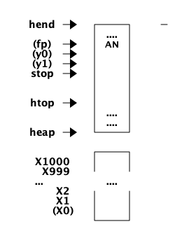
除 x 和 y 寄存器外,还有一些特殊功能寄存器:
-
Htop - The top of the heap.(堆顶)
-
E - The top of the stack. (栈顶)
-
CP - Continuation Pointer, i.e. function return address (接续点)
-
I - instruction pointer (指令指针)
-
fcalls - reduction counter (规约值计数器)
这些寄存器是 PCB 中相应字段的缓存版本。
    {move,{x,0},{x,1}}. % x1 := x0 (id(A))
    {move,{y,0},{x,0}}. % x0 := y0 (B)
    {move,{x,1},{y,0}}. % y0 := x1 (id(A))
现在我们在 x0 中有了第二个参数 B (第一个参数寄存器),我们可以再次调用 id 函数 {call,1,{f,4}}。
在调用后,x0 包含 id(B),y0 包含 id(A),现在我们可以进行加法操作:{gc_bif,'+',{f,0},1,[{y,0},{x,0}],{x,0}}。(稍后我们将详细讨论 BIF 调用和 GC。)
5.2. 分派(Dispatch):直接线程代码
BEAM 中的指令译码器是用一种被称为直接线程( directly threaded )代码的技术实现的。在这个上下文中,线程 thread 这个词与操作系统线程、并发性或并行性没有任何关系。它是通过虚拟机本身线程化的执行路径。
如果我们看一下上文所示的处理算术表达式的朴素堆栈机,就会发现我们使用 Erlang 原子和模式匹配来解码要执行的指令。这是一个非常重的解码机器指令的机器。在实际机器中,我们将每条指令编码为一个 “机器字” 整数。
我们可以使用 C 语言,将堆栈机重写为 字节码( byte code )机。首先,我们重写编译器,使其产生字节码。这是非常直接的,只需将每条被编码为 atom 的指令替换为表示该指令的字节。为了能够处理大于 255 的整数,我们将整数编码为一个存储大小 ( size ) 的字节,后面接的是用字节编码的整数数值。
compile(Expression, FileName) ->
    [ParseTree] = element(2,
			  erl_parse:parse_exprs(
			    element(2,
				    erl_scan:string(Expression)))),
    file:write_file(FileName, generate_code(ParseTree) ++ [stop()]).

generate_code({op, _Line, '+', Arg1, Arg2}) ->
    generate_code(Arg1) ++ generate_code(Arg2) ++ [add()];
generate_code({op, _Line, '*', Arg1, Arg2}) ->
    generate_code(Arg1) ++ generate_code(Arg2) ++ [multiply()];
generate_code({integer, _Line, I}) -> [push(), integer(I)].

stop()     -> 0.
add()      -> 1.
multiply() -> 2.
push()     -> 3.
integer(I) ->
    L = binary_to_list(binary:encode_unsigned(I)),
    [length(L) | L].
现在让我们用 C 语言编写一个简单的虚拟机。完整的代码可以在 Appendix C 中找到。
#define STOP 0
#define ADD  1
#define MUL  2
#define PUSH 3

#define pop()   (stack[--sp])
#define push(X) (stack[sp++] = X)

int run(char *code) {
  int stack[1000];
  int sp = 0, size = 0, val = 0;
  char *ip = code;

  while (*ip != STOP) {
    switch (*ip++) {
    case ADD: push(pop() + pop()); break;
    case MUL: push(pop() * pop()); break;
    case PUSH:
      size = *ip++;
      val = 0;
      while (size--) { val = val * 256 + *ip++; }
      push(val);
      break;
    }
  }
  return pop();
}
你看,用 C 语言写的虚拟机不需要非常复杂。这台机器只是一个循环,通过查看指令指针 ( instruction pointer , ip) 指向的值来检查每条指令的字节码。
对于每个字节码指令,它将通过指令字节码分支跳转,跳到对应指令的 case 上执行指令。这需要对指令进行解码,然后跳转到正确的代码上。如果我们看一下vsm.c (gcc -S vsm.c) 的汇编指令,我们可以看到解码器的内部循环:
L11:
        movl    -16(%ebp), %eax
        movzbl  (%eax), %eax
        movsbl  %al, %eax
        addl    $1, -16(%ebp)
        cmpl    $2, %eax
        je      L7
        cmpl    $3, %eax
        je      L8
        cmpl    $1, %eax
        jne     L5
它必须将字节代码与每个指令代码进行比较,然后执行条件跳转。在一个指令集中有许多指令的真实机器中,这可能会变得相当昂贵。
更好的解决方案是有一个包含代码地址的表,这样我们就可以在表中使用索引来加载地址并跳转,而不需要进行比较。这种技术有时称为 标记线程代码 ( token threaded code )。更进一步,我们可以将实现指令的函数的地址存储在代码内存中。这叫做 子程序线程代码 ( subroutine threaded code )。
这种方法将使在运行时解码更简单,但它使整个VM更加复杂,因为它需要一个加载器。加载程序将字节代码指令替换为实现指令的函数的地址。
一个加载器可能看起来像这样:
typedef void (*instructionp_t)(void);

instructionp_t *read_file(char *name) {
  FILE *file;
  instructionp_t *code;
  instructionp_t *cp;
  long  size;
  char ch;
  unsigned int val;

  file = fopen(name, "r");

  if(file == NULL) exit(1);

  fseek(file, 0L, SEEK_END);
  size = ftell(file);
  code = calloc(size, sizeof(instructionp_t));
  if(code == NULL) exit(1);
  cp = code;

  fseek(file, 0L, SEEK_SET);
  while ( ( ch = fgetc(file) ) != EOF )
    {
      switch (ch) {
      case ADD: *cp++ = &add; break;
      case MUL: *cp++ = &mul; break;
      case PUSH:
	*cp++ = &pushi;
	ch = fgetc(file);
	val = 0;
	while (ch--) { val = val * 256 + fgetc(file); }
	*cp++ = (instructionp_t) val;
	break;
      }
    }
  *cp = &stop;

  fclose(file);
  return code;
}
正如我们所看到的,我们在加载时做了更多的工作,包括对大于255的整数进行解码。(是的,我知道,以上代码对于非常大的整数是不安全的。)
如此,解码和分派循环的VM变得相当简单:
int run() {
  sp = 0;
  running = 1;

  while (running) (*ip++)();

  return pop();
}
然后我们只需要实现这些指令:
void add()  { int x,y; x = pop(); y = pop(); push(x + y); }
void mul()  { int x,y; x = pop(); y = pop(); push(x * y); }
void pushi(){ int x;   x = (int)*ip++;       push(x); }
void stop() { running = 0; }
在 BEAM 中,这个概念更进一步,BEAM使用直接线程代码(directly threaded code 有时也被称为 thread code )。在直接线程代码中,调用和返回序列被直接跳转到下一条指令的实现所取代。为了在 C 语言中实现这一点,BEAM 使用了 GCC "labels as values" 扩展。
稍后我们将进一步研究 BEAM 模拟器,但我们将快速了解 add 指令是如何实现的。由于大量使用宏,代码有些难以理解。这个 STORE_ARITH_RESULT 宏实际上隐藏了一个看起来像:I += 4; Goto(*I); 的分派函数。
#define OpCase(OpCode)    lb_##OpCode
#define Goto(Rel) goto *(Rel)

...

 OpCase(i_plus_jId):
 {
     Eterm result;

     if (is_both_small(tmp_arg1, tmp_arg2)) {
     Sint i = signed_val(tmp_arg1) + signed_val(tmp_arg2);
     ASSERT(MY_IS_SSMALL(i) == IS_SSMALL(i));
     if (MY_IS_SSMALL(i)) {
         result = make_small(i);
         STORE_ARITH_RESULT(result);
     }

     }
     arith_func = ARITH_FUNC(mixed_plus);
     goto do_big_arith2;
 }
为了让我们更容易理解 BEAM 分派器是如何实现的,让我们举一个更形象的例子。我们将从一些真正的 external BEAM 代码开始,然后我会发明一些 internal BEAM 指令,并用 C 实现它们。
如果我们从 Erlang 中一个简单的 add 函数开始:
add(A,B) -> id(A) + id(B).编译为 BEAM 码后如下:
{function, add, 2, 2}.
  {label,1}.
    {func_info,{atom,add},{atom,add},2}.
  {label,2}.
    {allocate,1,2}.
    {move,{x,1},{y,0}}.
    {call,1,{f,4}}.
    {move,{x,0},{x,1}}.
    {move,{y,0},{x,0}}.
    {move,{x,1},{y,0}}.
    {call,1,{f,4}}.
    {gc_bif,'+',{f,0},1,[{y,0},{x,0}],{x,0}}.
    {deallocate,1}.
    return.
(完整代码见 Appendix C 中的 add.erl 和 add.S。)
现在,如果我们聚焦这段代码中函数调用的三条指令:
    {move,{x,0},{x,1}}.
    {move,{y,0},{x,0}}.
    {move,{x,1},{y,0}}.
这段代码首先将函数调用 (x0) 的返回值保存在一个新的寄存器 (x1) 中。然后,它将调用者保存寄存器 (y0) 移动到第一个参数寄存器 (x0)。最后,它将 x1 中保存的值移动到调用者保存寄存器 (y0) ,以便在下一个函数调用时依旧存活。
假设我们要在 BEAM 中实现三条指令 move_xx, move_yx, 和 move_xy ( 这些指令在 BEAM 中不存在,我们只是用它们来演示这个例子):
#define OpCase(OpCode)    lb_##OpCode
#define Goto(Rel) goto *((void *)Rel)
#define Arg(N) (Eterm *) I[(N)+1]


  OpCase(move_xx):
  {
     x(Arg(1)) = x(Arg(0));
     I += 3;
     Goto(*I);
  }

  OpCase(move_yx): {
    x(Arg(1)) = y(Arg(0));
    I += 3;
    Goto(*I);
  }


  OpCase(move_xy): {
    y(Arg(1)) = x(Arg(0));
    I += 3;
    Goto(*I);
}注意,goto * 中的星号并不意味着解引用,该表达式意味着跳转到地址指针,我们实际上应该将其写为 goto*。
现在假设这些指令的编译后的 C 代码最终被加载在内存地址 0x3000、0x3100 和 0x3200中。当 BEAM 码被加载时,三个移动指令中的代码将被执行指令的内存地址所取代。假设代码 ({move,{x,0},{x,1}}, {move,{y,0},{x,0}}, {move,{x,1},{y,0}}) 被加载到地址 0x1000:
                     /  0x1000: 0x3000 -> 0x3000: OpCase(move_xx): x(Arg(1)) = x(Arg(0))
{move,{x,0},{x,1}}  {   0x1004: 0x0                                I += 3;
                     \  0x1008: 0x1                                Goto(*I);
                     /  0x100c: 0x3100
{move,{y,0},{x,0}}  {   0x1010: 0x0
                     \  0x1014: 0x0
                     /  0x1018: 0x3200
{move,{x,1},{y,0}}  {   0x101c: 0x1
                     \  0x1020: 0x0
地址 0x1000 处的一个"字"指向 move_xx 指令的实现。如果寄存器 I 包含指向 0x1000 的指令指针,那么分派器将会去获取 *I( 即 0x3000 ) 并跳转到那个地址。 (goto* *I)
在 Chapter 7 中,我们将更深入地研究一些真实的 BEAM 指令以及它们是如何实现的。
5.3. 调度:非抢占,规约值计数
大多数现代多线程操作系统使用抢占式调度。这意味着操作系统决定何时从一个进程切换到另一个进程,而不管进程在做什么。这可以保护其他进程不受某个进程行为不当(例如:没有及时做出让步)的影响。
在使用非抢占式调度器的协作多任务中,运行的进程决定何时让步。这样做的好处是,让步过程可以在已知状态下完成。
例如,在像 Erlang 这样具有动态内存管理和类型标记值的语言中,实现可能被设计成只有在工作内存中没有 ”解除标记 ( untagged )“ 值时进程才会产生进程调度让步。
以 add 指令为例,要添加两个 Erlang 整数,仿真器首先必须解除对整数的标记(译注:值的类型标记被记录在变量所占内存中,要取得整数值,需要先把标签去除),然后将它们相加,然后将结果标记为(译注:增加标签)整数。如果使用了完全抢占式的调度程序,则无法保证在未标记整数时进程不会挂起。或者进程在堆上创建元组时被挂起,只剩下半个元组。这将使遍历挂起的进程堆栈和堆变得非常困难。
在语言级别上,所有进程都是并发运行的,程序员不应该处理显式的调度让步。BEAM 通过跟踪进程运行了多长时间来解决这个问题。这是通过计算规约值来实现的。这个术语最初来自于微积分中使用的数学术语:lambda 演算中使用的 beta-reduction。
BEAM 中规约值的定义并不是很明确,但我们可以把它看作是一小块工作,不会花太长时间 ( too long )。每个函数调用都被视为一次规约计数。BEAM 在进入每个函数时都要做一个测试,以检查进程是否耗尽了所有的规约值。如果有剩余的规约值,函数将被执行,否则进程将被挂起。
由于 Erlang 中没有循环,只有尾部递归函数调用,所以很难编写一个不消耗掉规约计数而完成大量工作的程序。
|
有些 BIFs 只使用 1 个规约计数就可以运行很长时间,比如 term_to_binary 和 binary_to_term。请确保调用这些BIFs时,只使用小项式或 binary,否则可能会将调度器锁定很长一段时间。 另外,如果您编写自己的 NIFs,请确保它们能够产生让步,并与运行时间成比例地使规约值减少。 |
我们将在 Chapter 11 中详细介绍调度器的工作方式。
5.4. 内存管理:垃圾收集
Erlang 支持垃圾回收;作为 Erlang 程序员,您不需要执行显式内存管理。在 BEAM 层面,代码负责检查栈和堆溢出,并在栈和堆上分配足够的空间。
BEAM 指令 test_heap 将确保堆上有足够的空间满足需求。如果需要,该指令将调用垃圾收集器来回收堆上的空间。垃圾收集器将依次调用内存子系统的更底层实现来根据需要分配或释放内存。我们将在 Chapter 12 中详细介绍内存管理和垃圾收集。
5.5. BEAM: 一个虚拟机
BEAM 是一个虚拟机,也就是说它是用软件而不是硬件实现的。已经有项目通过 FPGA 实现 BEAM,同样也没有什么可以阻止任何人在硬件上实现 BEAM。一个更好的描述可能是称 BEAM 为一个抽象的机器,并把它看作可以执行 BEAM 代码的机器的蓝图。事实上,BEAM 中的 "AM" 两个字母就代表 “抽象机器”。
在本书中,我们将不区分抽象机器,虚拟机或它们的实现。在更正式的设定中,抽象机器是计算机的理论模型,虚拟机是抽象机器的软件实现,或者是真实物理机器的软件仿真器。
不幸的是,目前还没有关于 BEAM 的官方规范,它目前仅由 Erlang/OTP 中的实现定义。如果您想实现您自己的 BEAM,您就必须尝试模拟当前的实现,而不知道哪些部分是必要的,哪些部分是偶然的。你必须模仿每一个可观察的行为,以确保你有一个有效的 BEAM 解释器。
6. 模块和 BEAM 文件格式
6.1. 模块
| TODO 什么是模块 如何加载代码 热代码加载是如何工作的 净化(purging)是如何工作的 代码服务器(code server) 是如何工作的 动态代码加载如何工作,代码搜索路径 在分布式系统中处理代码。(与第10章重叠,要看什么去哪里。) 参数化模块 p-mod是如何实现的 p-mod调用的技巧 |
以下是本手稿的一段摘录:
6.2. BEAM 文件格式
关于 beam 文件格式的确切信息来源显然是 beam_lib.erl (参见 https://github.com/erlang/otp/blob/maint/lib/stdlib/src/beam_lib.erl)。实际上,还有一份由Beam的主要开发人员和维护人员编写的关于该格式的描述(参见 http://www.erlang.se/~bjorn/beam_file_format.html),可读性更好,但有些过时。
BEAM 文件格式基于交换文件格式 (interchange file format, EA IFF)#,有两个小的变化。我们将这些不久。IFF文件以文件头开始,后面跟着许多“块”。在IFF规范中有许多主要处理图像和音乐的标准块类型。但是IFF标准也允许您指定自己的命名块,而这正是 BEAM 所做的。
注意:Beam文件与标准IFF文件不同,因为每个块是在4字节边界 (即32位字) 上对齐的,而不是在IFF标准中在2字节边界上对齐的。为了表明这不是一个标准的 IFF 文件,IFF 头被标记为 “FOR1” 而不是 “FOR”。IFF 规范建议将此标记用于未来的扩展。
Beam 使用的 form type 值为:“Beam”。一个 Beam 文件头有以下布局:
BEAMHeader = <<
  IffHeader:4/unit:8 = "FOR1",
  Size:32/big,                  // big endian, how many more bytes are there
  FormType:4/unit:8 = "BEAM"
>>
在文件头之后可以找到多个块。每个块的大小与4字节的倍数对齐,并且(每个块)都有自己的块头部 (见下面描述)。
注意:对齐对于某些平台很重要,在这些平台中,对于未对齐的内存字节访问将产生一个硬件异常(在Linux中称为SIGBUS)。这可能导致性能下降,或者异常可能导致VM崩溃。
BEAMChunk = <<
  ChunkName:4/unit:8,           // "Code", "Atom", "StrT", "LitT", ...
  ChunkSize:32/big,
  ChunkData:ChunkSize/unit:8,   // data format is defined by ChunkName
  Padding4:0..3/unit:8

>>
该文件格式在所有区域前加上这个区域的大小,使得在从磁盘读取文件时可以很容易地直接解析文件。为了说明beam文件的结构和内容,我们将编写一个程序,它能从一个 beam 文件中提取所有数据块。为了使这个程序尽可能简单和可读,我们不会在读取时解析文件,而是将整个文件作为二进制文件加载到内存中,然后解析每个块。第一步是得到所有块的列表:
-module(beamfile).
-export([read/1]).

read(Filename) ->
   {ok, File} = file:read_file(Filename),
   <<"FOR1",
     Size:32/integer,
     "BEAM",
     Chunks/binary>> = File,
   {Size, read_chunks(Chunks, [])}.

read_chunks(<<N,A,M,E, Size:32/integer, Tail/binary>>, Acc) ->
   %% Align each chunk on even 4 bytes
   ChunkLength = align_by_four(Size),
   <<Chunk:ChunkLength/binary, Rest/binary>> = Tail,
   read_chunks(Rest, [{[N,A,M,E], Size, Chunk}|Acc]);
read_chunks(<<>>, Acc) -> lists:reverse(Acc).

align_by_four(N) -> (4 * ((N+3) div 4)).
一次样例运行结果可能是这样的:
> beamfile:read("beamfile.beam").
{848,
[{"Atom",103,
  <<0,0,0,14,4,102,111,114,49,4,114,101,97,100,4,102,105,
    108,101,9,114,101,97,...>>},
 {"Code",341,
  <<0,0,0,16,0,0,0,0,0,0,0,132,0,0,0,14,0,0,0,4,1,16,...>>},
 {"StrT",8,<<"FOR1BEAM">>},
 {"ImpT",88,<<0,0,0,7,0,0,0,3,0,0,0,4,0,0,0,1,0,0,0,7,...>>},
 {"ExpT",40,<<0,0,0,3,0,0,0,13,0,0,0,1,0,0,0,13,0,0,0,...>>},
 {"LocT",16,<<0,0,0,1,0,0,0,6,0,0,0,2,0,0,0,6>>},
 {"Attr",40,
  <<131,108,0,0,0,1,104,2,100,0,3,118,115,110,108,0,0,...>>},
 {"CInf",130,
  <<131,108,0,0,0,4,104,2,100,0,7,111,112,116,105,111,...>>},
 {"Abst",0,<<>>}]}
其中,我们可以看到 beam 使用的块名称。
6.2.1. 原子表块
名为 Atom 或 AtU8 的数据块都是强制必须包含的。它包含了模块提到的所有原子。对于 latin1 编码的源文件,使用名为 Atom 的块。对于 utf8 编码的模块,块被命名为 AtU8 。atom 块的格式为:
AtomChunk = <<
  ChunkName:4/unit:8 = "Atom",
  ChunkSize:32/big,
  NumberOfAtoms:32/big,
  [<<AtomLength:8, AtomName:AtomLength/unit:8>> || repeat NumberOfAtoms],
  Padding4:0..3/unit:8
>>
AtU8块只有名称不同(为 AtU8 ),其他同 atom 块。
| 模块名称永远存储在原子表的第一个位置 (atom index 0)。 |
让我们为原子块添加一个解码器到我们的 BEAM 文件读取器:
-module(beamfile).
-export([read/1]).

read(Filename) ->
   {ok, File} = file:read_file(Filename),
   <<"FOR1",
     Size:32/integer,
     "BEAM",
     Chunks/binary>> = File,
   {Size, parse_chunks(read_chunks(Chunks, []),[])}.

read_chunks(<<N,A,M,E, Size:32/integer, Tail/binary>>, Acc) ->
   %% Align each chunk on even 4 bytes
   ChunkLength = align_by_four(Size),
   <<Chunk:ChunkLength/binary, Rest/binary>> = Tail,
   read_chunks(Rest, [{[N,A,M,E], Size, Chunk}|Acc]);
read_chunks(<<>>, Acc) -> lists:reverse(Acc).

parse_chunks([{"Atom", _Size,
             <<_Numberofatoms:32/integer, Atoms/binary>>}
            | Rest], Acc) ->
   parse_chunks(Rest,[{atoms,parse_atoms(Atoms)}|Acc]);
parse_chunks([Chunk|Rest], Acc) -> %% Not yet implemented chunk
   parse_chunks(Rest, [Chunk|Acc]);
parse_chunks([],Acc) -> Acc.

parse_atoms(<<Atomlength, Atom:Atomlength/binary, Rest/binary>>) when Atomlength > 0->
   [list_to_atom(binary_to_list(Atom)) | parse_atoms(Rest)];
parse_atoms(_Alignment) -> [].

align_by_four(N) -> (4 * ((N+3) div 4)).
6.2.2. 导出表块
名为 ExpT (EXPort Table) 的块是强制必须包含的,它包含关于该模块要导出哪些函数的信息。
导出块的格式为:
ExportChunk = <<
  ChunkName:4/unit:8 = "ExpT",
  ChunkSize:32/big,
  ExportCount:32/big,
  [ << FunctionName:32/big,
       Arity:32/big,
       Label:32/big
    >> || repeat ExportCount ],
  Padding4:0..3/unit:8
>>
FunctionName 是原子表中的索引。
我们可以通过在原子处理子句之后添加以下子句来扩展 parse_chunk 函数:
parse_chunks([{"ExpT", _Size,
             <<_Numberofentries:32/integer, Exports/binary>>}
            | Rest], Acc) ->
   parse_chunks(Rest,[{exports,parse_exports(Exports)}|Acc]);

…

parse_exports(<<Function:32/integer,
               Arity:32/integer,
               Label:32/integer,
               Rest/binary>>) ->
   [{Function, Arity, Label} | parse_exports(Rest)];
parse_exports(<<>>) -> [].
6.2.3. 导入表块
名为 ImpT (IMPort Table) 的块是强制必须包含的,它包含关于模块要导入哪些函数的信息。
数据块的格式为:
ImportChunk = <<
  ChunkName:4/unit:8 = "ImpT",
  ChunkSize:32/big,
  ImportCount:32/big,
  [ << ModuleName:32/big,
       FunctionName:32/big,
       Arity:32/big
    >> || repeat ImportCount ],
  Padding4:0..3/unit:8
>>
这里的 ModuleName 和 FunctionName 是原子表中的索引。
| 解析导入表的代码与解析导出表的代码类似,但并不完全相同:两者都是 32 位整数的三元组,只是它们的含义不同。请参阅本章末尾的完整代码。 |
6.2.4. 代码块
名为 Code 的块是强制必须包含的,它包含了 beam 代码。块的格式如下:
ImportChunk = <<
  ChunkName:4/unit:8 = "Code",
  ChunkSize:32/big,
  SubSize:32/big,
  InstructionSet:32/big,        % Must match code version in the emulator
  OpcodeMax:32/big,
  LabelCount:32/big,
  FunctionCount:32/big,
  Code:(ChunkSize-SubSize)/binary,  % all remaining data
  Padding4:0..3/unit:8
>>
字段 SubSize 存储代码开始前的字数量。这使得在代码块中添加新的信息字段而不破坏旧的加载器成为可能。
InstructionSet 字段指示文件使用哪个版本的指令集。如果任何指令以不兼容的方式更改,版本号就会增加。
OpcodeMax 字段表示代码中使用的所有操作码的最大数量。即使新指令被添加到系统中,只要文件中使用的指令在加载器知道的范围内,旧的加载器仍然可以加载新文件。
字段 LabelCount 包含标签的数量,以便加载器可以通过一次调用就将标签表按照正确的大小预分配好。字段 FunctionCount 包含函数的数量,这样函数表也可以有效地预分配空间。
Code 字段包含连接在一起的指令,其中每个指令有以下格式:
Instruction = <<
  InstructionCode:8,
  [beam_asm:encode(Argument) || repeat Arity]
>>
这里, Arity 硬编码在表格中,当模拟器从源码构造 beam 码时,表格是由 genop 脚本的 ops.tab 生成的。(译注:此处如果不能够理解,可以参考 Chapter 9)
由 beam_asm:encode 产生的编码在下面的 [SEC-BeamModulesCTE,紧凑的项式编码] 节中进行了解释。
我们可以通过在程序中添加以下代码来解析代码块:
parse_chunks([{"Code", Size, <<SubSize:32/integer,Chunk/binary>>
              } | Rest], Acc) ->
   <<Info:SubSize/binary, Code/binary>> = Chunk,
   %% 8 is size of CunkSize & SubSize
   OpcodeSize = Size - SubSize - 8,
   <<OpCodes:OpcodeSize/binary, _Align/binary>> = Code,
   parse_chunks(Rest,[{code,parse_code_info(Info), OpCodes}
                      | Acc]);

..

parse_code_info(<<Instructionset:32/integer,
		  OpcodeMax:32/integer,
		  NumberOfLabels:32/integer,
		  NumberOfFunctions:32/integer,
		  Rest/binary>>) ->
   [{instructionset, Instructionset},
    {opcodemax, OpcodeMax},
    {numberoflabels, NumberOfLabels},
    {numberofFunctions, NumberOfFunctions} |
    case Rest of
	 <<>> -> [];
	 _ -> [{newinfo, Rest}]
    end].
我们将在后面的章节中( [beam_instructions] )学习如何解码 beam 指令。
6.2.5. 字符串表块
名为 StrT 的块是强制的,它包含模块中的所有常量字符串,并作为一个长字符串。如果模块中没有字符串字面量,块应该仍然存在,但为空且大小为0。
数据块的格式为:
StringChunk = <<
  ChunkName:4/unit:8 = "StrT",
  ChunkSize:32/big,
  Data:ChunkSize/binary,
  Padding4:0..3/unit:8
>>
字符串块可以很容易地解析,只需将字符串字节转换为二进制 (binary):
parse_chunks([{"StrT", _Size, <<Strings/binary>>} | Rest], Acc) ->
    parse_chunks(Rest,[{strings,binary_to_list(Strings)}|Acc]);
6.2.6. 属性块
名为 Attr 的数据块是可选的,但一些 OTP 工具希望属性块存在。发布处理程序期望 "vsn" 属性存在。您可以通过: beam_lib:version(Filename) 从文件中获得 version 属性,该函数假设存在一个属性块,其中包含一个 "vsn" 属性。
属性块的格式为:
AttributesChunk = <<
  ChunkName:4/unit:8 = "Attr",
  ChunkSize:32/big,
  Attributes:ChunkSize/binary,
  Padding4:0..3/unit:8
>>
我们可以使用如下方法解析属性块:
parse_chunks([{"Attr", Size, Chunk} | Rest], Acc) ->
    <<Bin:Size/binary, _Pad/binary>> = Chunk,
    Attribs = binary_to_term(Bin),
    parse_chunks(Rest,[{attributes,Attribs}|Acc]);
6.2.7. 编译信息块
名为 CInf 的数据块是可选的,但一些 OTP 工具希望编译信息块存在。
编译信息块的格式为:
CompilationInfoChunk = <<
  ChunkName:4/unit:8 = "CInf",
  ChunkSize:32/big,
  Data:ChunkSize/binary,
  Padding4:0..3/unit:8
>>
我们可以像这样解析编译信息块:
parse_chunks([{"CInf", Size, Chunk} | Rest], Acc) ->
    <<Bin:Size/binary, _Pad/binary>> = Chunk,
    CInfo = binary_to_term(Bin),
    parse_chunks(Rest,[{compile_info,CInfo}|Acc]);
6.2.8. 局部函数表块
名为 LocT 的块是可选的,用于交叉引用工具。
局部函数表块的格式与导出表相同:
LocalFunTableChunk = <<
  ChunkName:4/unit:8 = "LocT",
  ChunkSize:32/big,
  FunctionCount:32/big,
  [ << FunctionName:32/big,
       Arity:32/big,
       Label:32/big
    >> || repeat FunctionCount ],
  Padding4:0..3/unit:8
>>| 解析本地函数表的代码与解析导出和导入表的代码基本相同,实际上我们可以使用相同的函数来解析所有表中的条目。请参阅本章末尾的完整代码。 |
6.2.9. 字面值表块
名为 LitT 的块是可选的,它以压缩形式包含来自模块源文件的所有字面值,这些字面值不是即时(immediate) 值。块的格式为:
LiteralTableChunk = <<
  ChunkName:4/unit:8 = "LitT",
  ChunkSize:32/big,
  UncompressedSize:32/big,      % It is nice to know the size to allocate some memory
  CompressedLiterals:ChunkSize/binary,
  Padding4:0..3/unit:8
>>
其中 压缩文字 (CompressedLiterals) 必须有精确的 非压缩大小 (UncompressedSize) 字节。表中的每个字面值都用外部项式格式 (erlang:term_to_binary) 编码。 CompressedLiterals 的格式如下:
CompressedLiterals = <<
  Count:32/big,
  [ <<Size:32/big, Literal:binary>>  || repeat Count ]

>>
整个表用 zlib:compress/1 压缩,也可以用 zlib:uncompress/1 解压缩。
我们可以这样解析块:
parse_chunks([{"LitT", _ChunkSize,
              <<_CompressedTableSize:32, Compressed/binary>>}
             | Rest], Acc) ->
    <<_NumLiterals:32,Table/binary>> = zlib:uncompress(Compressed),
    Literals = parse_literals(Table),
parse_chunks(Rest,[{literals,Literals}|Acc]);…
parse_literals(<<Size:32,Literal:Size/binary,Tail/binary>>) ->
    [binary_to_term(Literal) | parse_literals(Tail)];
parse_literals(<<>>) -> [].
6.2.10. 抽象代码块
名为 Abst 的块是可选的,可以以抽象形式包含代码。如果将 debug_info 标记给编译器,它将在此块中存储模块的抽象语法树。像 debugger 和 Xref 这样的 OTP 工具需要抽象代码块。数据块的格式为:
AbstractCodeChunk = <<
  ChunkName:4/unit:8 = "Abst",
  ChunkSize:32/big,
  AbstractCode:ChunkSize/binary,
  Padding4:0..3/unit:8
>>
我们可以这样解析块:
parse_chunks([{"Abst", _ChunkSize, <<>>} | Rest], Acc) ->
    parse_chunks(Rest,Acc);
parse_chunks([{"Abst", _ChunkSize, <<AbstractCode/binary>>} | Rest], Acc) ->
parse_chunks(Rest,[{abstract_code,binary_to_term(AbstractCode)}|Acc]);6.2.12. 函数跟踪块 (已过时)
函数跟踪块(Function Trace chuck) 类型目前已经过时了。
6.2.14. 紧凑的项式编码
让我们看看 beam_asm:encode 时使用的算法。BEAM 文件以一种节省空间的方式使用一种特殊编码在 BEAM 文件中存储简单的项式。它不同于 VM 所使用的内存项式布局。
Beam_asm 是 compiler 应用程序中的一个模块,它是Erlang发行版的一部分,用于组装 beam 模块的二进制内容。
|
这种复杂设计背后的原因是:试图在第一个字节中放入尽可能多的类型和值数据,以使代码段更紧凑。解码后,所有编码值成为全尺寸机器字或项式。

自OTP 20 以来,这个标签格式已经改变, Extended - Float 消失了。下面所有的标签值向下移动1: List 是 2#10111,fpreg 是 2#100111,alloc List 是 2#110111,literal 是 2#1010111。浮点值现在直接进入 BEAM 文件的文字区域 (literal area)。
|
它使用第一个字节的前3位来存储定义以下值类型的标记。如果这些位都是1 (特殊值7或 beam_opcodes.hrl 中的 ?tag_z),那么会使用更多的位。
对于16以下的值,将值完全置于4-5-6-7位中,并将位3设为0:

对于 2048 (16#800) 以下的值,3 位被设置为 1,表示将使用 1 个延续字节,并且值的 3 个最有效 (significant) 位将扩展到这个字节的 5-6-7 位:

较大的值和负值首先被转换为字节。如果值需要 2 到 8 个字节,3-4 位将被设置为 1,5-6-7 位将包含值的 (bytes -2) 大小,如下:

如果下面的值大于 8 字节,那么所有的位 3-4-5-6-7 将被设置为1,后面跟着一个嵌套的编码无符号字面值( beam_opcodes.hrl 中的宏 ?tag_u ) 值为 (Bytes-9):8,接下来是数据字节:

标签类型
当读取压缩项式格式时,根据 Tag 的值可能会对结果整数进行不同的解释。
-
对于字面值,值是到字面值表的索引。
-
对于原子,值为原子索引数 减 1。如果值为0,则表示
NIL(空列表)。 -
标签 0 表示无效值。
-
如果标记为字符,则值为无符号 unicode 码点。
-
标签扩展列表包含项式对。读取
Size,创建Size的元组,然后能读取到Size/2个项式对。每一对分别是ValueandLabel。其中Value是用来进行比较的项式,Label是用来进行匹配的。这在select_val指令中使用。
请参考编译器应用程序中的 beam_asm:encode/2 ,以了解更多关于如何进行编码的细节。标签值在本节中给出,但也可以在 compiler/src/beam_opcodes.hrl 中找到。
7. 通用 BEAM 指令集
Beam 有两种不同的指令集,一种是内部指令集,称为 specific 特殊指令集,另一种是外部指令集,称为 generic 通用指令集。
通用指令集可以被称为官方指令集,这也是编译器和 Beam 解释器都使用的指令集。如果有一个官方的 Erlang 虚拟机规范,它会指定这个指令集为官方指令集。如果你想编写自己的运行在 Beam 的程序编译器,这是你应该生成的目标指令集。如果您想编写自己的 EVM,这是您应该处理的指令集。
外部指令集非常稳定,但是在 Erlang 版本之间,特别是在主要版本之间,它也会发生变化。
这是我们将在本章中介绍的指令集。
另一个指令集 (specific) 是 Beam 用来实现外部指令集的优化指令集。为了让你理解 Beam 是如何工作的,我们将在 Chapter 10 中介绍这个指令集。内部指令集可以在次要版本之间甚至在补丁版本之间更改而不发出警告。任何基于内部指令集的工具都是有风险的。
在这一章中,我将详细介绍这些指令的一般语法和一些指令组,Appendix B 中有一个完整的带有简短描述的指令列表。
7.1. 指令定义
通用指令的名称和操作码在 lib/compiler/src/genop.tab 中被定义。
该文件包含 Beam 指令格式的版本号,该版本号也被写入 .beam 文件中。这个数字到目前为止没有改变,仍然是版本0。如果外部格式将以非向后兼容的方式更改,则此数字将更改。
beam_makeops 是一个从 ops tabs 生成代码的 perl 脚本,它使用 genop.tab 作为输入。生成器在为编译器生成 Erlang 代码 (beam_opcodes.hrl 和 beam_opcodes.erl)的同时,也为仿真器生成C代码(TODO: 是什么??)。
文件中任何以 "#" 开头的行都是注释,会被 beam_makeops 忽略。该文件可以包含以下形式的定义,这些定义在perl脚本中转换为绑定:
NAME=EXPR
例如:
BEAM_FORMAT_NUMBER=0
“Beam 格式编号”与”外部 Beam 格式“中的 instructionset 字段相同。只有在对指令集进行向后不兼容的更改时才会发生改变。
文件的主要内容是如下形式的操作码定义:
OPNUM: [-]NAME/ARITY
OPNUM 和 ARITY 是整数,NAME 是一个以小写字母(a-z) 开头的标识符,而 ":","-" 和 "/" 是字面值 ( literals )。
例如:
1: label/1
负号 (-) 表示已经弃用而不建议使用的函数。已弃用的函数保留其操作码,以便加载器能够向后兼容 (它将识别已弃用的指令并拒绝加载代码)。
在本章的其余部分,我们将详细介绍一些 BEAM 指令。完整的列表和简要描述见:Appendix B 。
7.2. BEAM 代码清单
正如我们在 Chapter 2 中看到的那样,我们可以向 Erlang 编译器提供选项 'S',以人为和机器可读的格式(实际上是以 Erlang 项式的形式) 获取带有模块 BEAM 代码的 .S 文件。
给定文件 beamexample1.erl:
-module(beamexample1).

-export([id/1]).

id(I) when is_integer(I) -> I.
当用 erlc -S beamexample 编译时。我们得到了下面的 beamexmaple.S 文件:
{module, beamexample1}.  %% version = 0

{exports, [{id,1},{module_info,0},{module_info,1}]}.

{attributes, []}.

{labels, 7}.


{function, id, 1, 2}.
  {label,1}.
    {line,[{location,"beamexample1.erl",5}]}.
    {func_info,{atom,beamexample1},{atom,id},1}.
  {label,2}.
    {test,is_integer,{f,1},[{x,0}]}.
    return.


{function, module_info, 0, 4}.
  {label,3}.
    {line,[]}.
    {func_info,{atom,beamexample1},{atom,module_info},0}.
  {label,4}.
    {move,{atom,beamexample1},{x,0}}.
    {line,[]}.
    {call_ext_only,1,{extfunc,erlang,get_module_info,1}}.


{function, module_info, 1, 6}.
  {label,5}.
    {line,[]}.
    {func_info,{atom,beamexample1},{atom,module_info},1}.
  {label,6}.
    {move,{x,0},{x,1}}.
    {move,{atom,beamexample1},{x,0}}.
    {line,[]}.
    {call_ext_only,2,{extfunc,erlang,get_module_info,2}}.
实际的 beam 代码中,除了 id/1 函数,我们也得到一些元指令。
第一行 {module, beamexample1}. %% version = 0 告诉我们模块名称是"beamexample1",指令集的版本号为 "0"。
然后我们得到一个导出函数的列表 "id/1, module_info/0, module_info/1"。我们可以看到,编译器向代码中添加了两个自动生成的函数。这两个函数只是通用模块信息 BIF ( erlang:module_info/1 和 erlang:module_info/2)的分派器,其中添加了模块的名称作为第一个参数。
行 {attributes, []} 列出了所有已定义的编译器属性,在我们的例子中没有。
然后我们知道在模块中只有不到 7 个标签,{labels, 7} 这一行使得一次加载代码变得很容易。
最后一种元指令是格式为 {function, Name, Arity, StartLabel} 的 function 指令。正如我们在 id/1 函数中看到的,开始标签实际上是函数代码中的第二个标签。
{label, N} ”指令“ 实际上不是一条指令,它在加载时不会占用内存中的任何空间。它只是为代码中的位置提供一个本地名称(或数字)。每个 label 都标记块的开始,因为每个 label 都可能是跳转的潜在目标。
第一个标签 ( {label,1} )之后的前两个指令实际上是为报错生成的代码,它添加行号、模块、函数和参数目信息,并抛出异常。即 line 和 func_info 指令。
在 {label,2} 之后,指令 {test,is_integer,{f,1},[{x,0}]} 才是函数的”肉“。test 指令测试它的参数 (在末尾的列表中,在本例中是变量{x,0}) 是否满足测试,在本例中是一个整数测试 (is_integer)。如果测试成功,则执行下一条指令 ( return )。否则,函数将失败,并跳转到 label 1 ({f,1}),也就是说,在 label 1 处继续执行,此时会抛出函数子句异常。
文件中的其他两个函数是自动生成的。如果我们查看第二个函数,则指令 {move,{x,0},{x,1}} 将寄存器 x0 中的参数移动到第二个参数寄存器 x1 中。然后指令 {move,{atom,beamexample1},{x,0}} 将模块名 atom 移动到第一个参数寄存器 x0。最后对 erlang:get_module_info/2 进行一个尾部调用 ({call_ext_only,2,{extfunc,erlang,get_module_info,2}})。正如我们将在下一节中看到的,有几种不同的调用指令。
7.3. 调用 (call)
正如我们在 Chapter 8 中看到的,Erlang 中有几种不同类型的调用。为了区分指令集中的本地调用和远程调用,远程调用的指令名中有 _ext。本地调用只有模块代码中的一个标签,而远程调用的目标形式为 {extfunc, Module, Function, Arity}。
为了区分普通(堆栈构建)调用和尾部递归调用,后者的名称中有 _only 或者 _last 。带 _last 的变体还将尽可能多的释放由最后一个参数给出的堆栈槽。
还有一个 call_fun Arity 指令,它调用寄存器 {x, Arity} 中存储的闭包。参数存储在 x0 到 {x, array -1} 中。
所有类型的调用指令的完整清单见 Appendix B。
7.4. 栈 (堆) 管理
在 Beam 上的 Erlang 进程的栈和堆共享相同的内存区域,请参阅 Chapter 3 和 Chapter 12 以获得完整的讨论。堆栈向低地址增长,堆向高地址增长。如果新的空间需求超出堆栈当前可提供的空间,Beam 将执行垃圾收集。
在进入非叶子函数时,CP指针 ( continuation pointer ) 被保存在栈上,在退出时,它被从堆栈读回。这是由 allocate 和 deallocate 指令完成的,它们用于为当前指令设置和拆除栈帧。
叶函数的函数框架是这样的:
{function, Name, Arity, StartLabel}.
  {label,L1}.
    {func_info,{atom,Module},{atom,Name},Arity}.
  {label,L2}.
    ...
    return.
一个非叶函数的函数框架是这样的:
{function, Name, Arity, StartLabel}.
  {label,L1}.
    {func_info,{atom,Module},{atom,Name},Arity}.
  {label,L2}.
    {allocate,Need,Live}.

    ...
    call ...
    ...

    {deallocate,Need}.
    return.
指令 allocate StackNeed Live 保存 CP 指针( continuation pointer ) ,并在栈上为 StackNeed 分配额外空间。如果在分配期间需要GC,则需要保存 Live 个 X 寄存器。例如,如果 Live 是 2,那么寄存器 X0 和 X1 将被保存。
在栈上分配空间时,栈指针 (E) 将被减小。

所有类型的分配 ( allocate ) 和释放 ( deallocate ) 指令的完整清单见 Appendix B。
7.5. 消息传递
用 beam 码发送信息非常直接。你只需要使用 send 指令。注意尽管发送指令不带任何参数,它更像是一个函数调用。它假设参数 (目的地和消息) 在参数寄存器 X0 和 X1 中。消息也被从 X1 复制到 X0。
接收消息要稍微复杂一些,因为它既涉及带有模式匹配的选择性接收,又在函数体中引入一个 yield / resume 点。(还有一个特性可以使用 refs 最小化消息队列扫描,稍后将对此进行详细介绍。)
7.5.1. 最小接收循环
一个最小的接收循环,它接受任何消息并且没有超时 (例如:receive _ -> ok end ),在 BEAM 代码中是这样的:
A minimal receive loop, which accepts any message and has no timeout (e.g. receive _ -> ok end) looks like this in BEAM code:
  {label,2}.
    {wait,{f,1}}.
  {label,1}.
    {loop_rec,{f,2},{x,0}}.
    remove_message.
    {jump,{f,3}}.
  {label,2}.
    {wait,{f,1}}.
  {label,3}.
     ...
+loop_rec L2 x0+ 指令首先检查消息队列中是否有消息。如果没有消息执行跳转到L2,在那里进程将被挂起等待消息到达。
如果消息队列中有消息,则 loop_rec 指令还将该消息从 m-buf 移动到进程堆中。有关 m-buf 处理的详细信息,请参阅 Chapter 12 和 Chapter 3。
对于像 receive _ -> ok end 这样的代码,我们接受任何消息,且不需要模式匹配,我们只需要执行一个 remove_message 来从消息队列中将本消息与下一条消息分离。(它还消除了任何超时,稍后将详细介绍。)
7.5.2. 选择性接收循环
对于一个选择性接收,例如 receive [] -> ok end ,我们将在消息队列循环检查队列中是否有匹配的消息。
  {label,1}.
    {loop_rec,{f,3},{x,0}}.
    {test,is_nil,{f,2},[{x,0}]}.
    remove_message.
    {jump,{f,4}}.
  {label,2}.
    {loop_rec_end,{f,1}}.
  {label,3}.
    {wait,{f,1}}.
  {label,4}.
    ...
在本例中,如果邮箱中有消息,我们在 loop_rec 指令之后对 Nil 执行模式匹配。如果消息不匹配,我们会在 L3 结束,其中 loop_rec_end 指令将保存指针指向到下一个消息 (p->msg.save = &(*p->msg.save)->next) ,并跳转回 L2。
如果消息队列中没有更多消息,则进程将被位于 L4 的 wait 指令挂起,保存指针将指向消息队列的末尾。当进程被重新调度时,它将只查看消息队列中的新消息 (保存点之后)。
7.5.3. 带超时的接收循环
如果我们向选择性接收添加一个超时,那么 wait 指令将被一个 wait_timeout 指令取代,后面跟着一个超时指令和超时之后要执行的代码。
  {label,1}.
    {loop_rec,{f,3},{x,0}}.
    {test,is_nil,{f,2},[{x,0}]}.
    remove_message.
    {jump,{f,4}}.
  {label,2}.
    {loop_rec_end,{f,1}}.
  {label,3}.
    {wait_timeout,{f,1},{integer,1000}}.
    timeout.
  {label,4}.
    ...
wait_timeout 指令用给定的时间 (在我们的示例中是 1000 毫秒) 设置一个超时计时器,它还在 p->def_arg_reg[0] 保存了下一条指令的地址 ( timeout ),然后当计时器被设置后,将 p->i 设置为指向 def_arg_reg。
这意味着当进程挂起时,如果没有匹配的消息到达,1 秒后超时将被触发,进程将在超时指令处继续执行指令。
注意,如果邮箱中接收到不匹配的消息,进程将被调度执行,并将在接收循环中运行模式匹配代码,但不会取消超时。因为超时计时器的取消是在 remove_message 中执行的。
超时指令将邮箱的保存点重置为队列中的第一个元素,并从 PCB 中清除超时标志 (F_TIMO)。
7.5.4. 同步调用的技巧 ( Ref Trick )
现在我们已经到了接收循环的最后一个版本,我们使用前面提到的 ref 技巧来避免长信箱扫描。
Erlang 代码中的一种常见模式是实现一种远程调用 "remote call" ,在两个进程之间进行消息的发送和接收。例如 gen_server 中就是这样用的。这种代码通常隐藏在一个用普通函数调用包装过的库之后。例如,你调用函数 counter:increment(Counter) ,在这个场景的背后,它变成了类似 Counter ! {self(), inc}, receive {Counter, Count} -> Count end。
这通常是封装进程中状态的很好的抽象。不过,当调用进程的邮箱中有许多消息时,会出现一个小问题。在这种情况下,receive 必须检查邮箱中的每条消息,以确定除最后一条消息外没有任何消息与返回消息匹配。
如果您的服务器接收了许多消息,并且对于每个消息执行了许多此类远程调用,那么这种情况经常会发生,如果没有适当的反压,服务器消息队列将被填满。
为了补救这个问题,在 ERTS 中有一个技巧可以识别这个模式,并避免扫描整个消息队列来寻找返回消息。
编译器识别在接收中使用新创建的引用 (ref) 的代码 ( 参见 [ref_trick_code]),并输出能避免长时间的收件箱扫描的代码,因为新的引用不可能已经在收件箱中。
  Ref = make_ref(),
  Counter ! {self(), inc, Ref},
  receive
    {Ref, Count} -> Count
  end.
这为我们提供了以下完整接收的框架,请参见 [ref_receive]。
    {recv_mark,{f,3}}.
    {call_ext,0,{extfunc,erlang,make_ref,0}}.
    ...
    send.
    {recv_set,{f,3}}.
  {label,3}.
    {loop_rec,{f,5},{x,0}}.
    {test,is_tuple,{f,4},[{x,0}]}.
    ...
    {test,is_eq_exact,{f,4},[{x,1},{y,0}]}.
    ...
    remove_message.
    ...
    {jump,{f,6}}.
  {label,4}.
    {loop_rec_end,{f,3}}.
  {label,5}.
    {wait,{f,3}}.
  {label,6}.
recv_mark 指令在 msg.saved_last 中保存当前位置( msg.last ),在 msg.mark 中保存 label 地址。
recv_set 指令检查 msg.mark 是否指向下一条指令,如果指向下一条指令,将保存点 ( msg.save ) 移动到创建 ref (msg.saved_last) 之前收到的最后一条消息。如果 msg.mark 无效 (即不等于 msg.save),则指令不执行任何操作。
8. 各种类型的调用,链接以及热代码加载(原书未完成)
8.1. 热代码加载
在 Erlang 中,本地函数调用和远程函数调用之间存在语义上的差异。远程调用 (即对已命名模块中的函数的调用) 保证会转到该模块的最新加载版本。本地调用 (对同一模块内的函数的非限定调用) 保证会与调用转到相同的代码版本。
通过在调用点指定模块名称,可以将对本地函数的调用转换为远程调用。这通常通过 ?MODULE 宏来完成,如 ?MODULE:foo() 。对非本地模块的远程调用不能转换为本地调用,也就是说,无法在调用者中保证被调用者的版本。
这是 Erlang 的一个重要特性,它使得热代码加载或热升级成为可能。只要确保你在服务器循环的某个地方有一个远程调用,然后你可以在系统运行时加载这个远程调用函数的新代码;当执行到达远程调用时,它将切换为执行新代码。
写服务器循环的一种常见方式是有一个本地调用的主循环和一个代码升级处理程序,升级处理程序负责做一个远程调用和可能的状态升级:
loop(State) ->
  receive
    upgrade ->
       NewState = ?MODULE:code_upgrade(State),
       ?MODULE:loop(NewState);
     Msg ->
       NewState = handle_msg(Msg, State),
       loop(NewState)
   end.
使用这个构造,也就是 gen_server 使用的基本构造,程序员可以控制何时以及如何进行代码升级。
热代码升级是 Erlang 最重要的特性之一,它使编写全天候运行的服务器成为可能。这也是 Erlang 是动态类型的主要原因之一。在静态类型语言中,为 code_upgrade 函数指定类型是非常困难的。(也很难给出循环函数的类型)。这些类型将在未来随着状态类型的改变而改变,以处理新特性。
语言实现者关心性能问题,热代码加载功能是一种负担。由于对远程模块的每次调用或从远程模块调用都可能在将来更改为新代码,因此跨模块边界进行整个程序优化非常困难。(这很难,但并非不可能,有解决方案,但迄今为止我还没有看到一个全面实施的案例)。
8.2. 代码加载
在 Erlang 运行时系统中,代码加载由代码服务器 (code server) 处理。代码服务器将调用 erlang 模块中的更底层 BIFs 来进行实际加载。但是代码服务器也决定清除策略。
运行时系统可以保存每个模块的两个版本,一个是当前版本,一个是旧版本。所有完全限定 (远程) 调用都转到当前版本。旧版本中的本地函数调用和堆栈上的返回地址仍然可以转到旧版本函数。
如果加载了模块的第三个版本,并且仍然有进程在运行 (在堆栈上有指向旧代码的指针) 旧代码,代码服务器将杀死那些进程并清除旧代码。然后,当前版本将变成旧代码,第三个版本将作为当前版本加载。
9. BEAM 加载器
9.1. 从通用指令变换为特定指令
BEAM 加载器不只是获取外部 BEAM 格式并将其写入内存。它还对代码进行许多变换,并将外部 (通用) 格式转换为内部 (特定) 格式。
加载器的代码可以在 beam_load.c (在 erts/emulator/beam ) 中找到,但是大多数翻译逻辑都在文件 ops.tab (在 erts/emulator/beam/emu ) 中。
加载器的第一步是解析 beam 文件,基本上和我们在 Chapter 6 中使用 Erlang 所做的工作相同,但是该程序是用 C 编写的。
然后是 ops.tab 中的规则被应用于代码块 (译注:code chuck, 见 Section 6.2.4 ) 中的指令,以将通用指令转换为一个或多个特定指令。
翻译表通过模式匹配工作。文件中的每一行都定义了一个或多个带参数的通用指令的模式,可选的一个箭头(译注:"⇒" 符号),后面跟着一个或多个要转换的指令。
ops tab 中的转换尝试处理编译器生成的指令模式,通过窥孔优化将它们优化为更少的特定指令。ops tab 转换尝试为选择的模式生成跳转表。
ops.tab 文件并不是在运行时解析的,而是从 ops.tab 生成一个模式匹配程序,并存储在生成的一个 C 文件中的数组中。perl 脚本 beam_makeops (在 erts/emulator/utils 中) 在 beam_opcodes.h 和 beam_opcodes.c 文件中生成一组特定于目标的操作码和翻译程序(这些文件在给定的目标目录中,例如 erts/emulator/x86_64-unknown-linux-gnu/opt/smp/)。
同一个程序 (beam_makeops) 还为编译器后端 beam_opcodes.erl 生成 Erlang 代码。
9.2. 理解 ops.tab
ops.tab 中的变换按照它们写入文件的顺序执行。因此,就像在 Erlang 模式匹配中一样,不同规则的触发顺序是自上而下的。
在 ops.tab 中的指令参数的类型可以在 Appendix B 中可以找到。
9.2.1. 变换
ops.tab 中的大多数规则是不同指令之间的变换。一个简单的变换是这样的:
move S x==0 | return => move_return S
这组合了从任何位置移动到 x(0) 的 move 指令和 return 指令,成为一个名为 move_return 的单指令。让我们把变换分开看看不同的部分做了什么。
- move
-
is the instruction that the pattern first has to match. This can be either a generic instruction that the compiler has emitted, or a temporary instruction that
ops.tabhas emitted to help with transformations. - S
-
is a variable binding any type of value. Any value in the pattern (left hand side or
⇒) that is used in the generator (right hand side of⇒) has to be bound to a variable. - x==0
-
is a guard that says that we only apply the transformation if the target location is an
xregister with the value0. It is possible to chain multiple types and also bind a variable here. For instanceD=xy==0would allow bothxandyregisters with a value of0and also bind the argument to the variableD. - |
-
signifies the end of this instruction and the beginning of another instruction that is part of the same pattern.
- return
-
is the second instruction to match in this pattern.
⇒-
signifies the end of the pattern and the start of the code that is to be generated.
- move_return S
-
is the name of the generated instruction together with the name of the variable on the lhs. It is possible to generate multiple instructions as part of a transformation by using the
|symbol.
More complex translations can be done in ops.tab. For instance take the
select_val
instruction. It will be translated by the loader into either a jump table, a linear
search array or a binary search array depending on the input values.
is_integer Fail=f S | select_val S=s Fail=f Size=u Rest=* | \
  use_jump_tab(Size, Rest) => gen_jump_tab(S, Fail, Size, Rest)
The above transformation creates a jump table if possible of the select_val.
There are a bunch of new techniques used in the transformations.
- S
-
is used in both
is_integerandselect_val. This means that both the values have to be of the same type and have the same value. Furthermore theS=sguard limits the type to a be a source register. - Rest=*
-
allows a variable number of arguments in the instruction and binds them to variable
Rest. - use_jump_tab(Size, Rest)
-
calls the use_jump_tab C function in
beam_load.cthat decides whether the arguments in theselect_valcan be transformed into a jump table. - \
-
signifies that the transformation rule continues on the next line.
- gen_jump_tab(S, Fail, Size, Rest)
-
calls the gen_jump_tab C function in
beam_load.cthat takes care of generating the appropriate instruction.
9.2.2. 特定指令
When all transformations are done, we have to decide how the specifc instruction should
look like. Let’s continue to look at move_return:
%macro: move_return MoveReturn -nonext
move_return x
move_return c
move_return n
This will generate three different instructions that will use the
MoveReturn
macro in beam_emu.c to do the work.
- %macro: move_return
-
this tells
ops.tabto generate the code formove_return. If there is no%macroline, the instruction has to be implemented by hand in beam_emu.c. The code for the instruction will be places inbeam_hot.horbeam_cold.hdepending on if the%hotor%colddirective is active. - MoveReturn
-
tells the code generator to that the name of the c-macro in beam_emu.c to use is MoveReturn. This macro has to be implemented manually.
- -nonext
-
tells the code generator that it should not generate a dispatch to the next instruction, the
MoveReturnmacro will take care of that. - move_return x
-
tells the code generator to generate a specific instruction for when the instruction argument is an x register.
cfor when it is a constant,nwhen it isNIL. No instructions are in this case generated for when the argument is a y register as the compiler will never generate such code.
The resulting code in beam_hot.h will look like this:
OpCase(move_return_c):
    {
    MoveReturn(Arg(0));
    }

OpCase(move_return_n):
    {
    MoveReturn(NIL);
    }

OpCase(move_return_x):
    {
    MoveReturn(xb(Arg(0)));
    }
All the implementor has to do is to define the MoveReturn macro in beam_emu.c and
the instruction is complete.
The %macro rules can take multiple different flags to modify the code that
gets generated.
The examples below assume that there is a specific instructions looking like this:
%macro move_call MoveCall
move_call x f
without any flags to the %macro we the following code will be generated:
BeamInstr* next;
PreFetch(2, next);
MoveCall(Arg(0));
NextPF(2, next);| The PreFetch and NextPF macros make sure to load the address to jump to next before the instruction is executed. This trick increases performance on all architectures by a variying amount depending on cache architecture and super scalar properties of the CPU. |
- -nonext
-
Don’t emit a dispatch for this instructions. This is used for instructions that are known to not continue with the next instructions, i.e. return, call, jump.
%macro move_call MoveCall -nonext
MoveCall(xb(Arg(0)));- -arg_*
-
Include the arguments of type * as arguments to the c-macro. Not all argument types are included by default in the c-macro. For instance the type
fused for fail labels and local function calls is not included. So giving the option-arg_fwill include that as an argument to the c-macro.
%macro move_call MoveCall -arg_f
MoveCall(xb(Arg(0)), Arg(1));- -size
-
Include the size of the instruction as an argument to the c-macro.
%macro move_call MoveCall -size
MoveCall(xb(Arg(0)), 2);- -pack
-
Pack any arguments if possible. This places multiple register arguments in the same word if possible. As register arguments can only be 0-1024, we only need 10 bits to store them + 2 for tagging. So on a 32-bit system we can put 2 registers in one word, while on a 64-bit we can put 4 registers in one word. Packing instruction can greatly decrease the memory used for a single instruction. However there is also a small cost to unpack the instruction, which is why it is not enabled for all instructions.
The example with the call cannot do any packing as f cannot be packed and only one
other argument exists. So let’s look at the
put_list
instruction as an example instead.
%macro:put_list PutList -pack
put_list x x x
BeamInstr tmp_packed1;
BeamInstr* next;
PreFetch(1, next);
tmp_packed1 = Arg(0);
PutList(xb(tmp_packed1&BEAM_TIGHT_MASK),
        xb((tmp_packed1>>BEAM_TIGHT_SHIFT)&BEAM_TIGHT_MASK),
        xb((tmp_packed1>>(2*BEAM_TIGHT_SHIFT))));
NextPF(1, next);
This packs the 3 arguments into 1 machine word, which halves the required memory for this instruction.
- -fail_action
-
Include a fail action as an argument to the c-macro. Note that the
ClauseFail()macro assumes the fail label is in the first argument of the instructions, so in order to use this in the above example we should transform themove_call x ftomove_call f x.
%macro move_call MoveCall -fail_action
MoveCall(xb(Arg(0)), ClauseFail());- -gen_dest
-
Include a store function as an argument to the c-macro.
%macro move_call MoveCall -gen_dest
MoveCall(xb(Arg(0)), StoreSimpleDest);- -goto
-
Replace the normal next dispatch with a jump to a c-label inside beam_emu.c
%macro move_call MoveCall -goto:do_call
MoveCall(xb(Arg(0)));
goto do_call;
9.3. 优化
加载器在加载代码时执行许多窥孔优化。其中最重要的是指令组合和指令专门化。
指令组合是将两条或多条较小的指令合并成一条较大的指令。如果已知这些指令大部分时间都是相互跟随的,那么这可能会导致代码的速度大大加快。之所以能够加快速度,是因为不再需要在指令之间执行分派 ( dispatch,译注:参见 Section 5.2 ),而且 C 编译器在优化指令时可以获得更多信息。何时执行指令组合是一种权衡,必须考虑主仿真器循环增大的大小与执行指令时的增益之间的影响。
指令专门化消除了对指令中的参数进行解码的需要。因此,用已经解码的参数生成的将不是一条 move_sd ,而是 move_xx, move_xy 等指令。这减少了指令的解码成本,但这也是对仿真器代码大小的权衡考量。
9.3.1. select_val 优化
编译器生成 select_val 指令来对许多函数或 case 子句进行控制流处理。例如:
select(1) -> 3;
select(2) -> 3;
select(_) -> error.
编译为:
{function, select, 1, 2}.
  {label,1}.
    {line,[{location,"select.erl",5}]}.
    {func_info,{atom,select},{atom,select},1}.
  {label,2}.
    {test,is_integer,{f,4},[{x,0}]}.
    {select_val,{x,0},{f,4},{list,[{integer,2},{f,3},{integer,1},{f,3}]}}.
  {label,3}.
    {move,{integer,3},{x,0}}.
    return.
  {label,4}.
    {move,{atom,error},{x,0}}.
    return.
The values in the condition are only allowed to be either integers
or atoms. If the value is of any other type the compiler will not emit a
select_val instruction. The loader uses a couple of hearistics to figure
out what type algorithm to use when doing the select_val.
- jump_on_val
-
Create a jump table and use the value as the index. This if very efficient and happens when a group of close together integers are used as the value to select on. If not all values are present, the jump table is padded with extra fail label slots.
- select_val2
-
Used when only two values are to be selected upon and they to not fit in a jump table.
- select_val_lins
-
Do a linear search of the sorted atoms or integers. This is used when a small amount of atoms or integers are to be selected from.
- select_val_bins
-
Do a binary search of the sorted atoms or integers.
9.3.2. 字面值预哈希
当加载一个字面值并将其用作任何需要字面值 hash 值的 bifs 或指令的参数时,该 hash 值由加载器创建并由指令使用,而不是每次都对字面值进行 hash。
使用这种技术的代码示例有 maps 指令和进程字典 (PD) bifs。
10. BEAM 内部指令(原书未完成)
空白,原书未完成
11. Scheduling
To fully understand where time in an ERTS system is spent you need to understand how the system decides which Erlang code to run and when to run it. These decisions are made by the Scheduler.
The scheduler is responsible for the real-time guarantees of the system. In a strict Computer Science definition of the word real-time, a real-time system has to be able to guarantee a response within a specified time. That is, there are real deadlines and each task has to complete before its deadline. In Erlang there are no such guarantees, a timeout in Erlang is only guaranteed to not trigger before the given deadline.
In a general system like Erlang where we want to be able to handle all sorts of programs and loads, the scheduler will have to make some compromises. There will always be corner cases where a generic scheduler will behave badly. After reading this chapter you will have a deeper understanding of how the Erlang scheduler works and especially when it might not work optimally. You should be able to design your system to avoid the corner cases and you should also be able to analyze a misbehaving system.
11.1. Concurrency, Parallelism, and Preemptive Multitasking
Erlang is a concurrent language. When we say that processes run concurrently we mean that for an outside observer it looks like two processes are executing at the same time. In a single core system this is achieved by preemptive multitasking. This means that one process will run for a while, and then the scheduler of the virtual machine will suspend it and let another process run.
In a multicore or a distributed system we can achieve true parallelism, that is, two or more processes actually executing at the exact same time. In an SMP enabled emulator the system uses several OS threads to indirectly execute Erlang processes by running one scheduler and emulator per thread. In a system using the default settings for ERTS there will be one thread per enabled core (physical or hyper threaded).
We can check that we have a system capable of parallel execution, by checking if SMP support is enabled:
iex(1)> :erlang.system_info :smp_support
true
We can also check how many schedulers we have running in the system:
iex(2)> :erlang.system_info :schedulers_online
4
We can see this information in the Observer as shown in the figure below.
If we spawn more processes than schedulers we have and
let them do some busy work we can see that there are a number
of processes running in parallel and some processes that
are runnable but not currently running. We can see this
with the function erlang:process_info/2.
1> Loop = fun (0, _) -> ok; (N, F) -> F(N-1, F) end,
   BusyFun = fun() -> spawn(fun () -> Loop(1000000, Loop) end) end,
   SpawnThem = fun(N) -> [ BusyFun() || _ <- lists:seq(1, N)] end,
   GetStatus = fun() -> lists:sort([{erlang:process_info(P, [status]), P}
                        || P <- erlang:processes()]) end,
   RunThem = fun (N) -> SpawnThem(N), GetStatus() end,
   RunThem(8).

[{[{status,garbage_collecting}],<0.62.0>},
 {[{status,garbage_collecting}],<0.66.0>},
 {[{status,runnable}],<0.60.0>},
 {[{status,runnable}],<0.61.0>},
 {[{status,runnable}],<0.63.0>},
 {[{status,runnable}],<0.65.0>},
 {[{status,runnable}],<0.67.0>},
 {[{status,running}],<0.58.0>},
 {[{status,running}],<0.64.0>},
 {[{status,waiting}],<0.0.0>},
 {[{status,waiting}],<0.1.0>},

...
We will look closer at the different statuses that a process can have later in this chapter, but for now all we need to know is that a process that is running or garbage_collecting is actually running in on a scheduler. Since the machine in the example has four cores and four schedulers there are four process running in parallel (the shell process and three of the busy processes). There are also five busy processes waiting to run in the state runnable.
By using the Load Charts tab in the Observer we can see that all four schedulers are fully loaded while the busy processes execute.
observer:start().
ok
3> RunThem(8).
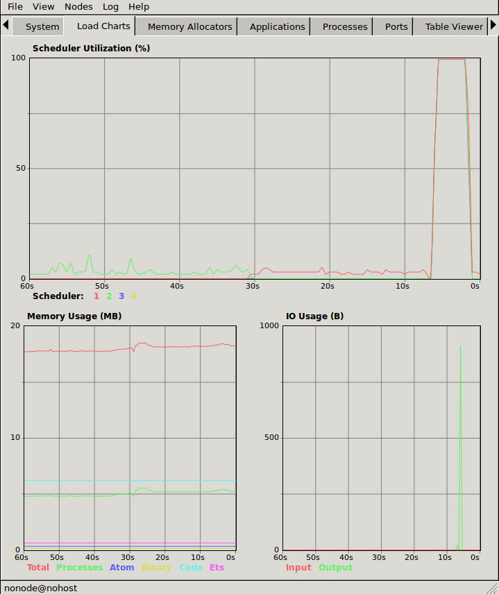
11.2. Preemptive Multitasking in ERTS Cooperating in C
The preemptive multitasking on the Erlang level is achieved by cooperative multitasking on the C level. The Erlang language, the compiler and the virtual machine works together to ensure that the execution of an Erlang process will yield within a limited time and let the next process run. The technique used to measure and limit the allowed execution time is called reduction counting, we will look at all the details of reduction counting soon.
11.3. Reductions
One can describe the scheduling in BEAM as preemptive scheduling on top of cooperative scheduling. A process can only be suspended at certain points of the execution, such as at a receive or a function call. In that way the scheduling is cooperative---a process has to execute code which allows for suspension. The nature of Erlang code makes it almost impossible for a process to run for a long time without doing a function call. There are a few Built In Functions (BIFs) that still can take too long without yielding. Also, if you call C code in a badly implemented Native Implemented Function (NIF) you might block one scheduler for a long time. We will look at how to write well behaved NIFs in Chapter 16.
Since there are no other loop constructs than recursion and
list comprehensions,
there is no way to loop forever without doing a function call.
Each function call is counted as a reduction; when the reduction
limit for the process is reached it is suspended.
|
Version Info
Prior to OTP-20.0, the value of |
|
Reductions
The term reduction comes from the Prolog ancestry of Erlang. In Prolog each execution step is a goal-reduction, where each step reduces a logic problem into its constituent parts, and then tries to solve each part. |
11.3.1. How Many Reductions Will You Get?
When a process is scheduled it will get a number of reductions defined
by CONTEXT_REDS (defined in
erl_vm.h,
currently as 4000). After using up its reductions or when doing a
receive without a matching message in the inbox, the process will be
suspended and a new processes will be scheduled.
If the VM has executed as many reductions as defined by
INPUT_REDUCTIONS (currently 2*CONTEXT_REDS, also defined in
erl_vm.h) or if there is no process ready to run
the scheduler will do system-level activities. That is, basically,
check for IO; we will cover the details soon.
11.3.2. What is a Reduction Really?
It is not completely defined what a reduction is, but at least each function call should be counted as a reduction. Things get a bit more complicated when talking about BIFs and NIFs. A process should not be able to run for "a long time" without using a reduction and yielding. A function written in C can not yield in the middle, it has to make sure it is in a clean state and return. In order to be re-entrant it has to save its internal state somehow before it returns and then set up the state again on re-entry. This can be very costly, especially for a function that sometimes only does little work and sometimes lot. The reason for writing a function in C instead of Erlang is usually to achieve performance and to not do unnecessary book keeping work. Since there is no clear definition of what one reduction is, other than a function call on the Erlang level, there is a risk that a function implemented in C takes many more clock cycles per reduction than a normal Erlang function. This can lead to an imbalance in the scheduler, and even starvation.
For example in Erlang versions prior to R16, the BIFs
binary_to_term/1 and term_to_binary/1 were non yielding and only
counted as one reduction. This meant that a process calling these
functions on large terms could starve other processes. This can even
happen in a SMP system because of the way processes are balanced
between schedulers, which we will get to soon.
While a process is running the emulator keeps the number of reductions
left to execute in the (register mapped) variable FCALLS (see
beam_emu.c).
We can examine this value with hipe_bifs:show_pcb/1:
iex(13)> :hipe_bifs.show_pcb self
 P: 0x00007efd7c2c0400
 -----------------------------------------------------------------
 Offset| Name          |              Value |             *Value |
     0 | id            | 0x00000270000004e3 |                    |

 ...

   328 | rcount        | 0x0000000000000000 |                    |
   336 | reds          | 0x000000000000a528 |                    |

 ...

   320 | fcalls        | 0x00000000000004a3 |                    |
The field reds keep track of the total number of reductions a
process has done up until it was last suspended. By monitoring this
number you can see which processes do the most work.
You can see the total number of reductions for a process (the reds
field) by calling erlang:process_info/2 with the atom reductions
as the second argument. You can also see this number in the process
tab in the observer or with the i/0 command in the Erlang shell.
As noted earlier, each time a process starts the field fcalls is set to
the value of CONTEXT_REDS and for each function call the
process executes fcalls is reduced by 1. When the process is
suspended the field reds is increased by the number of executed
reductions. In some C like code something like:
p→reds += (CONTEXT_REDS - p→fcalls).
Normally a process would do all its allotted reductions and fcalls
would be 0 at this point, but if the process suspends in a receive
waiting for a message it will have some reductions left.
When a process uses up all its reductions it will yield to let another process run, it will go from the process state running to the state runnable, if it yields in a receive it will instead go into the state waiting (for a message). In the next section we will take a look at all the different states a process can be in.
11.4. The Process State (or status)
The field status in the PCB contains the process state. It can be one
of free, runnable, waiting, running, exiting, garbing,
and suspended. When a process exits it is marked as
free---you should never be able to see a process in this state,
it is a short lived state where the process no longer exist as
far as the rest of the system is concerned but there is still
some clean up to be done (freeing memory and other resources).
Each process status represents a state in the Process State Machine. Events such as a timeout or a delivered message triggers transitions along the edges in the state machine. The Process State Machine looks like this:

The normal states for a process are runnable, waiting, and running. A running process is currently executing code in one of the schedulers. When a process enters a receive and there is no matching message in the message queue, the process will become waiting until a message arrives or a timeout occurs. If a process uses up all its reductions, it will become runnable and wait for a scheduler to pick it up again. A waiting process receiving a message or a timeout will become runnable.
Whenever a process needs to do garbage collection, it will go into
the garbing
state until the GC is done. While it is doing GC
it saves the old state in the field gcstatus and when it is done
it sets the state back to the old state using gcstatus.
The suspended state is only supposed to be used for debugging
purposes. You can call erlang:suspend_process/2 on another process
to force it into the suspended state. Each time a process calls
suspend_process on another process, the suspend count is increased.
This is recorded in the field rcount.
A call to (erlang:resume_process/1) by the suspending process will
decrease the suspend count. A process in the suspend state will not
leave the suspend state until the suspend count reaches zero.
The field rstatus (resume status) is used to keep track of the
state the process was in before a suspend. If it was running
or runnable it will start up as runnable, and if it was waiting
it will go back to the wait queue. If a suspended waiting process
receives a timeout rstatus is set to runnable so it will resume
as runnable.
To keep track of which process to run next the scheduler keeps the processes in a queue.
11.5. Process Queues
The main job of the scheduler is to keep track of work queues, that is, queues of processes and ports.
There are two process states that the scheduler has to handle, runnable, and waiting. Processes waiting to receive a message are in the waiting state. When a waiting process receives a message the send operations triggers a move of the receiving process into the runnable state. If the receive statement has a timeout the scheduler has to trigger the state transition to runnable when the timeout triggers. We will cover this mechanism later in this chapter.
11.5.1. The Ready Queue
Processes in the runnable state are placed in a FIFO (first in first out) queue handled by the scheduler, called the ready queue. The queue is implemented by a first and a last pointer and by the next pointer in the PCB of each participating process. When a new process is added to the queue the last pointer is followed and the process is added to the end of the queue in an O(1) operation. When a new process is scheduled it is just popped from the head (the first pointer) of the queue.
 The Ready Queue

 First: -->  P5       +---> P3       +-+-> P17
             next: ---+     next: ---+ |  next: NULL
                                       |
 Last: --------------------------------+
In a SMP system, where you have several scheduler threads, there is one queue per scheduler.
 Scheduler 1       Scheduler 2      Scheduler 3      Scheduler 4

 Ready: P5         Ready: P1        Ready: P7        Ready: P9
        P3                P4               P12
        P17                                P10
The reality is slightly more complicated since Erlang processes have priorities. Each scheduler actually has three queues. One queue for max priority tasks, one for high priority tasks and one queue containing both normal and low priority tasks.
 Scheduler 1       Scheduler 2      Scheduler 3      Scheduler 4

 Max:    P5        Max:             Max:             Max:
 High:             High:  P1        High:            High:
 Normal: P3        Ready: P4        Ready: P7        Ready: P9
         P17                               P12
                                           P10
If there are any processes in the max queue the scheduler will pick these processes for execution. If there are no processes in the max queue but there are processes in the high priority queue the scheduler will pick those processes. Only if there are no processes in the max and the high priority queues will the scheduler pick the first process from the normal and low queue.
When a normal process is inserted into the queue it gets a schedule count of 1 and a low priority process gets a schedule count of 8. When a process is picked from the front of the queue its schedule count is reduced by one, if the count reaches zero the process is scheduled, otherwise it is inserted at the end of the queue. This means that low priority processes will go through the queue seven times before they are scheduled.
11.5.2. Waiting, Timeouts and the Timing Wheel
A processs trying to do a receive on an empty mailbox or on a mailbox with no matching messages will yield and go into the waiting state.
When a message is delivered to an inbox the sending process will check whether the receiver is sleeping in the waiting state, and in that case it will wake the process, change its state to runable, and put it at the end of the appropriate ready queue.
If the receive statement has a timeout clause a timer will be created for the process which will trigger after the specified timeout time. The only guarantee the runtime system gives on a timeout is that it will not trigger before the set time, it might be some time after the intended time before the process is scheduled and gets to execute.
Timers are handled in the VM by a timing wheel. That is, an array of time slots which wraps around. Prior to Erlang 18 the timing wheel was a global resource and there could be some contention for the write lock if you had many processes inserting timers into the wheel. Make sure you are using a later version of Erlang if you use many timers.
The default size (TIW_SIZE) of the timing wheel is 65536 slots (or 8192 slots if you have built the system for a small memory footprint). The current time is indicated by an index into the array (tiw_pos). When a timer is inserted into the wheel with a timeout of T the timer is inserted into the slot at (tiw_pos+T)%TIW_SIZE.
   0 1                                      65535
  +-+-+- ... +-+-+-+-+-+-+-+-+-+-+-+ ... +-+-----+
  | | |      | | | | | | |t| | | | |     | |     |
  +-+-+- ... +-+-+-+-+-+-+-+-+-+-+-+ ... +-+-----+
              ^           ^                       ^
              |           |                       |
           tiw_pos     tiw_pos+T               TIW_SIZE
The timer stored in the timing wheel is a pointer to an ErlTimer struct. See erl_time.h. If several timers are inserted into the same slot they are linked together in a linked list by the prev and next fields. The count field is set to T/TIW_SIZE
/*
** Timer entry:
*/
typedef struct erl_timer {
    struct erl_timer* next;	/* next entry tiw slot or chain */
    struct erl_timer* prev;	/* prev entry tiw slot or chain */
    Uint slot;			/* slot in timer wheel */
    Uint count;			/* number of loops remaining */
    int    active;		/* 1=activated, 0=deactivated */
    /* called when timeout */
    void (*timeout)(void*);
    /* called when cancel (may be NULL) */
    void (*cancel)(void*);
    void* arg;        /* argument to timeout/cancel procs */
} ErlTimer;
11.6. Ports
A port is an Erlang abstraction for a communication point with the world outside of the Erlang VM. Communications with sockets, pipes, and file IO are all done through ports on the Erlang side.
A port, like a process, is created on the same scheduler as the creating process. Also like processes ports use reductions to decide when to yield, and they also get to run for 4000 reductions. But since ports don’t run Erlang code there are no Erlang function calls to count as reductions, instead each port task is counted as a number of reductions. Currently a task uses a little more than 200 reductions per task, and a number of reductions relative to one thousands of the size of transmitted data.
A port task is one operation on a port, like opening, closing, sending a number of bytes or receiving data. In order to execute a port task the executing thread takes a lock on the port.
Port tasks are scheduled and executed in each iteration in the scheduler loop (see below) before a new process is selected for execution.
11.7. Reductions
When a process is scheduled it will get a number of reductions defined
by CONTEXT_REDS (defined in
erl_vm.h,
currently as 4000). After using up its reductions or when doing a
up its reductions or when doing a receive without a matching message
in the inbox, the process will be suspended and a new processes will
be scheduled.
If the VM has executed as many reductions as defined by
INPUT_REDUCTIONS (currently 2*CONTEXT_REDS, also defined in
erl_vm.h) or if there is no process ready to run the scheduler will
do system-level activities. That is, basically, check for IO; we will
cover the details soon.
It is not completely defined what a reduction is, but at least each function call should be counted as a reduction. Things get a bit more complicated when talking about BIFs and NIFs. A process should not be able to run for "a long time" without using a reduction and yielding. A function written in C can usually not yield at any time, and the reason for writing it in C is usually to achieve performance. In such functions a reduction might take longer which can lead to imbalance in the scheduler.
For example in Erlang versions prior to R16 the BIFs binary_to_term/1 and term_to_binary/1 where non yielding and only counted as one reduction. This meant that a process calling theses functions on large terms could starve other processes. This can even happen in a SMP system because of the way processes are balanced between schedulers, which we will get to soon.
While a process is running the emulator keeps the number of reductions left to execute in the (register mapped) variable FCALLS (see beam_emu.c).
11.8. The Scheduler Loop
Conceptually you can look at the scheduler as the driver of program execution in the Erlang VM. In reality, that is, the way the C code is structured, it is the emulator (process_main in beam_emu.c) that drives the execution and it calls the scheduler as a subroutine to find the next process to execute.
Still, we will pretend that it is the other way around, since it makes a nice conceptual model for the scheduler loop. That is, we see it as the scheduler picking a process to execute and then handing over the execution to the emulator.
Looking at it that way, the scheduler loop looks like this:
-
Update reduction counters.
-
Check timers
-
If needed check balance
-
If needed migrate processes and ports
-
Do auxiliary scheduler work
-
If needed check IO and update time
-
While needed pick a port task to execute
-
Pick a process to execute
11.9. Load Balancing
The current strategy of the load balancer is to use as few schedulers as possible without overloading any CPU. The idea is that you will get better performance through better memory locality when processes share the same CPU.
One thing to note though is that the load balancing done in the scheduler is between scheduler threads and not necessarily between CPUs or cores. When you start the runtime system you can specify how schedulers should be allocated to cores. The default behaviour is that it is up to the OS to allocated scheduler threads to cores, but you can also choose to bind schedulers to cores.
The load balancer assumes that there is one scheduler running on each core so that moving a process from a overloaded scheduler to an under utilized scheduler will give you more parallel processing power. If you have changed how schedulers are allocated to cores, or if your OS is overloaded or bad at assigning threads to cores, the load balancing might actually work against you.
The load balancer uses two techniques to balance the load, task stealing and migration. Task stealing is used every time a scheduler runs out of work, this technique will result in the work becoming more spread out between schedulers. Migration is more complicated and tries to compact the load to the right number of schedulers.
11.9.1. Task Stealing
If a scheduler run queue is empty when it should pick a new process to schedule the scheduler will try to steal work from another scheduler.
First the scheduler takes a lock on itself to prevent other schedulers to try to steal work from the current scheduler. Then it checks if there are any inactive schedulers that it can steal a task from. If there are no inactive schedulers with stealable tasks then it will look at active schedulers, starting with schedulers having a higher id than itself, trying to find a stealable task.
The task stealing will look at one scheduler at a time and try to steal the highest priority task of that scheduler. Since this is done per scheduler there might actually be higher priority tasks that are stealable on another scheduler which will not be taken.
The task stealing tries to move tasks towards schedulers with lower numbers by trying to steal from schedulers with higher numbers, but since the stealing also will wrap around and steal from schedulers with lower numbers the result is that processes are spread out on all active schedulers.
Task stealing is quite fast and can be done on every iteration of the scheduler loop when a scheduler has run out of tasks.
11.9.2. Migration
To really utilize the schedulers optimally a more elaborate migration strategy is used. The current strategy is to compact the load to as few schedulers as possible, while at the same time spread it out so that no scheduler is overloaded.
This is done by the function check_balance in erl_process.c.
The migration is done by first setting up a migration plan and then letting schedulers execute on that plan until a new plan is set up. Every 2000*CONTEXT_REDS reductions a scheduler calculates a migration path per priority per scheduler by looking at the workload of all schedulers. The migration path can have three different types of values: 1) cleared 2) migrate to scheduler # 3) immigrate from scheduler #
When a process becomes ready (for example by receiving a message or triggering a timeout) it will normally be scheduled on the last scheduler it ran on (S1). That is, if the migration path of that scheduler (S1), at that priority, is cleared. If the migration path of the scheduler is set to emigrate (to S2) the process will be handed over to that scheduler if both S1 and S2 have unbalanced run-queues. We will get back to what that means.
When a scheduler (S1) is to pick a new process to execute it checks to see if it has an immigration path from (S2) set. If the two involved schedulers have unbalanced run-queues S1 will steal a process from S2.
The migration path is calculated by comparing the maximum run-queues for each scheduler for a certain priority. Each scheduler will update a counter in each iteration of its scheduler loop keeping track of the maximal queue length. This information is then used to calculate an average (max) queue length (AMQL).
 Max
 Run Q
 Length
    5         o
              o
           o  o
Avg: 2.5 --------------
           o  o     o
    1      o  o     o

scheduler S1 S2 S3 S4
Then the schedulers are sorted on their max queue lengths.
 Max
 Run Q
 Length
    5               o
                    o
                 o  o
Avg: 2.5 --------------
              o  o  o
    1         o  o  o

scheduler S3 S4 S1 S2

           ^        ^
           |        |
          tix      fix
Any scheduler with a longer run queue than average (S1, S2) will be marked for emigration and any scheduler with a shorter max run queue than average (S3, S4) will be targeted for immigration.
This is done by looping over the ordered set of schedulers with two indices (immigrate from (fix)) and (emigrate to (tix)). In each iteration of the a loop the immigration path of S[tix] is set to S[fix] and the emigration path of S[fix] is set to S[tix]. Then tix is increased and fix decreased till they both pass the balance point. If one index reaches the balance point first it wraps.
In the example: * Iteration 1: S2.emigrate_to = S3 and S3.immigrate_from = S2 * Iteration 2: S1.emigrate_to = S4 and S4.immigrate_from = S1
Then we are done.
In reality things are a bit more complicated since schedulers can be taken offline. The migration planning is only done for online schedulers. Also, as mentioned before, this is done per priority level.
When a process is to be inserted into a ready queue and there is a migration path set from S1 to S2 the scheduler first checks that the run queue of S1 is larger than AMQL and that the run queue of S2 is smaller than the average. This way the migration is only allowed if both queues are still unbalanced.
There are two exceptions though where a migration is forced even when the queues are balanced or even imbalanced in the wrong way. In both these cases a special evacuation flag is set which overrides the balance test.
The evacuation flag is set when a scheduler is taken offline to ensure that no new processes are scheduled on an offline scheduler. The flag is also set when the scheduler detects that no progress is made on some priority. That is, if there for example is a max priority process which always is ready to run so that no normal priority processes ever are scheduled. Then the evacuation flag will be set for the normal priority queue for that scheduler.
12. The Memory Subsystem: Stacks, Heaps and Garbage Collection
Before we dive into the memory subsystem of ERTS, we need to have some basic vocabulary and understanding of the general memory layout of a program in a modern operating system. In this review section I will assume the program is compiled to an ELF executable and running on Linux on something like an IA-32/AMD64 architecture. The layout and terminology is basically the same for all operating systems that ERTS compile on.
A program’s memory layout looks something like this:
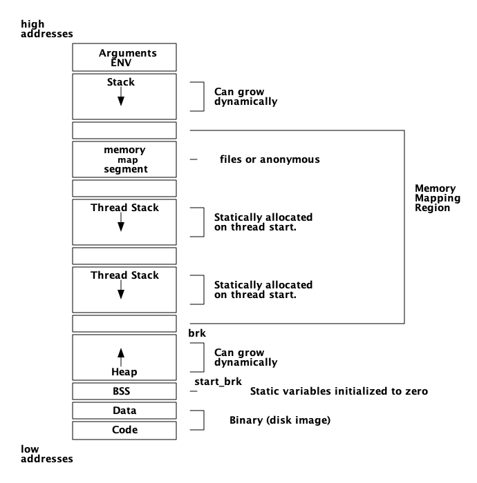
Even though this picture might look daunting it is still a simplification. (For a full understanding of the memory subsystem read a book like "Understanding the Linux Kernel" or "Linux System Programming") What I want you to take away from this is that there are two types of dynamically allocatable memory: the heap and memory mapped segments. I will try to call this heap the C-heap from now on, to distinguish it from an Erlang process heap. I will call a memory mapped segment for just a segment, and any of the stacks in this picture for the C-stack.
The C-heap is allocated through malloc and a segment is allocated with mmap.
-
A note on pictures of memory
12.1. The memory subsystem
Now that we dive into the memory subsystem it will once again be apparent that ERTS is more like an operating system than just a programming language environment. Not only does ERTS provide a garbage collector for Erlang terms on the Erlang process level, but it also provides a plethora of low level memory allocators and memory allocation strategies.
For an overview of memory allocators see the erts_alloc documentation at: http://www.erlang.org/doc/man/erts_alloc.html
All these allocators also comes with a number of parameters that can be used to tweak their behavior, and this is probably one of the most important areas from an operational point of view. This is where we can configure the system behavior to fit anything from a small embedded control system (like a Raspberry Pi) to an Internet scale 2TB database server.
There are currently eleven different allocators, six different allocation strategies, and more than 18 other different settings, some of which are taking arbitrary numerical values. This means that there basically is an infinite number of possible configurations. (OK, strictly speaking it is not infinite, since each number is bounded, but there are more configurations than you can shake a stick at.)
In order to be able to use these settings in any meaningful way we will have to understand how these allocators work and how each setting impacts the performance of the allocator.
The erts_alloc manual goes as far as to give the following warning:
Only use these flags if you are absolutely sure what you are doing. Unsuitable settings may cause serious performance degradation and even a system crash at any time during operation.
http://www.erlang.org/doc/man/erts_alloc.html
Making you absolutely sure that you know what you are doing, that is what this chapter is about.
Oh yes, we will also go into details of how the garbage collector works.
12.2. Different type of memory allocators
The Erlang run-time system is trying its best to handle memory in all situations and under all types of loads, but there are always corner cases. In this chapter we will look at the details of how memory is allocated and how the different allocators work. With this knoweledge and some tools that we will look at later you should be able to detect and fix problems if your system ends up in one of these corner cases.
For a nice story about the troubles the system might get into and how to analyze and correct the behavior read Fred Hébert’s essay "Troubleshooting Down the Logplex Rabbit Hole".
When we are talking about a memory allocator in this book we have a specific meaning in mind. Each memory allocator manage allocations and deallocations of memory of a certain type. Each allocator is intended for a specific type of data and is often specialized for one size of data.
Each memory allocator implements the allocator interface that can use different algorithms and settings for the actual memory allocation.
The goal with having different allocators is to reduce fragmentation, by grouping allocations of the same size, and to increase performance, by making frequent allocations cheap.
There are two special, fundamental or generic, memory allocator types sys_alloc and mseg_alloc, and nine specific allocators implemented through the alloc_util framework.
In the following sections we will go though the different allocators, with a little detour into the general framework for allocators (alloc_util).
Each allocator has several names used in the documentation and in the C code. See Table 1 for a short list of all allocators and their names. The C-name is used in the C-code to refer to the allocator. The Type-name is used in erl_alloc.types to bind allocation types to an allocator. The Flag is the letter used for setting parameters of that allocator when starting Erlang.
| Name | Description | C-name | Type-name | Flag |
|---|---|---|---|---|
Basic allocator |
malloc interface |
sys_alloc |
SYSTEM |
Y |
Memory segment allocator |
mmap interface |
mseg_alloc |
- |
M |
Temporary allocator |
Temporary allocations |
temp_alloc |
TEMPORARY |
T |
Heap allocator |
Erlang heap data |
eheap_alloc |
EHEAP |
H |
Binary allocator |
Binary data |
binary_alloc |
BINARY |
B |
ETS allocator |
ETS data |
ets_alloc |
ETS |
E |
Driver allocator |
Driver data |
driver_alloc |
DRIVER |
R |
Short lived allocator |
Short lived memory |
sl_alloc |
SHORT_LIVED |
S |
Long lived allocator |
Long lived memory |
ll_alloc |
LONG_LIVED |
L |
Fixed allocator |
Fixed size data |
fix_alloc |
FIXED_SIZE |
F |
Standard allocator |
For most other data |
std_alloc |
STANDARD |
D |
12.2.1. The basic allocator: sys_alloc
The allocator sys_alloc can not be disabled, and is basically a straight mapping to the underlying OS malloc implementation in libc.
If a specific allocator is disabled then sys_alloc is used instead.
All specific allocators uses either sys_alloc or mseg_alloc to allocate memory from the operating system as needed.
When memory is allocated from the OS sys_alloc can add (pad) a fixed number of kilobytes to the requested number. This can reduce the number of system calls by over allocating memory. The default padding is zero.
When memory is freed, sys_alloc will keep some free memory allocated in the process. The size of this free memory is called the trim threshold, and the default is 128 kilobytes. This also reduces the number of system calls at the cost of a higher memory footprint. This means that if you are running the system with the default settings you can experience that the Beam process does not give memory back to the OS directly as memory is freed up.
Memory areas allocated by sys_alloc are stored in the C-heap of the beam process which will grow as needed through system calls to brk.
12.2.2. The memory segment allocator: mseg_alloc
If the underlying operating system supports mmap a specific memory allocator can use mseg_alloc instead of sys_alloc to allocate memory from the operating system.
Memory areas allocated through mseg_alloc are called segments. When a segment is freed it is not immediately returned to the OS, instead it is kept in a segment cache.
When a new segment is allocated a cached segment is reused if possible, i.e. if it is the same size or larger than the requested size but not too large. The value of absolute max cache bad fit determines the number of kilobytes of extra size which is considered not too large. The default is 4096 kilobytes.
In order not to reuse a 4096 kilobyte segment for really small allocations there is also a relative_max_cache_bad_fit value which states that a cached segment may not be used if it is more than that many percent larger. The default value is 20 percent. That is a 12 KB segment may be used when asked for a 10 KB segment.
The number of entries in the cache defaults to 10 but can be set to any value from zero to thirty.
12.2.3. The memory allocator framework: alloc_util
Building on top of the two generic allocators (sys_alloc and mseg_alloc) is a framework called alloc_util which is used to implement specific memory allocators for different types of usage and data.
The framework is implemented in erl_alloc_util.[ch] and the different allocators used by ERTS are defined in erl_alloc.types in the directory "erts/emulator/beam/".
In a SMP system there is usually one allocator of each type per scheduler thread.
The smallest unit of memory that an allocator can work with is called a block. When you call an allocator to allocate a certain amount of memory what you get back is a block. It is also blocks that you give as an argument to the allocator when you want to deallocate memory.
The allocator does not allocate blocks from the operating system directly though. Instead the allocator allocates a carrier from the operating system, either through sys_alloc or through mseg_alloc, which in turn uses malloc or mmap. If sys_alloc is used the carrier is placed on the C-heap and if mseg_alloc is used the carrier is placed in a segment.
Small blocks are placed in a multiblock carrier. A multiblock carrier can as the name suggests contain many blocks. Larger blocks are placed in a singleblock carrier, which as the name implies on contains one block.
What’s considered a small and a large block is determined by the parameter singleblock carrier threshold (sbct), see the list of system flags below.
Most allocators also have one "main multiblock carrier" which is never deallocated.

Memory allocation strategies
To find a free block of memory in a multi block carrier an allocation strategy is used. Each type of allocator has a default allocation strategy, but you can also set the allocation strategy with the as flag.
The Erlang Run-Time System Application Reference Manual lists the following allocation strategies:
Best fit: Find the smallest block that satisfies the requested block size. (bf)
Address order best fit: Find the smallest block that satisfies the requested block size. If multiple blocks are found, choose the one with the lowest address. (aobf)
Address order first fit: Find the block with the lowest address that satisfies the requested block size. (aoff)
Address order first fit carrier best fit : Find the carrier with the lowest address that can satisfy the requested block size, then find a block within that carrier using the "best fit" strategy. (aoffcbf)
Address order first fit carrier address order best fit: Find the carrier with the lowest address that can satisfy the requested block size, then find a block within that carrier using the "address order best fit" strategy. aoffcaobf (address order first fit carrier address order best fit)
Good fit: Try to find the best fit, but settle for the best fit found during a limited search. (gf)
A fit: Do not search for a fit, inspect only one free block to see if it satisfies the request. This strategy is only intended to be used for temporary allocations. (af)
12.2.4. The temporary allocator: temp_alloc
The allocator temp_alloc, is used for temporary allocations. That is very short lived allocations. Memory allocated by temp_alloc may not be allocated over a Erlang process context switch.
You can use temp_alloc as a small scratch or working area while doing some work within a function. Look at it as an extension of the C-stack and free it in the same way. That is, to be on the safe side, free memory allocated by temp_alloc before returning from the function that did the allocation. There is a note in erl_alloc.types saying that you should free a temp_alloc block before the emulator starts executing Erlang code.
Note that no Erlang process running on the same scheduler as the allocator may start executing Erlang code before the block is freed. This means that you can not use a temporary allocation over a BIF or NIF trap (yield).
In a default R16 SMP system there is N+1 temp_alloc allocators where N is the number of schedulers. The temp_alloc uses the "A fit" (af) strategy. Since the allocation pattern of the temp_alloc basically is that of a stack (mostly of size 0 or 1), this strategy works fine.
The temporary allocator is, in R16, used by the following types of data: TMP_HEAP, MSG_ROOTS, ROOTSET, LOADER_TEMP, NC_TMP, TMP, DCTRL_BUF, TMP_DIST_BUF, ESTACK, DB_TMP, DB_MC_STK, DB_MS_CMPL_HEAP, LOGGER_DSBUF, TMP_DSBUF, DDLL_TMP_BUF, TEMP_TERM, SYS_READ_BUF, ENVIRONMENT, CON_VPRINT_BUF.
For an up to date list of allocation types allocated with each allocator, see erl_alloc.types (e.g. grep TEMPORARY erts/emulator/beam/erl_alloc.types).
I will not go through each of these different types, but in general as you can guess by their names, they are temporary buffers or work stacks.
12.2.5. The heap allocator: eheap_alloc
The heap allocator, is used for allocating memory blocks where tagged Erlang terms are stored, such as Erlang process heaps (all generations), heap fragments, and the beam_registers.
This is probably the memory areas you are most interested in as an Erlang developer or when tuning an Erlang system. We will talk more about how these areas are managed in the upcoming sections on garbage collection and process memory. There we will also cover what a heap fragment is.
12.2.6. The binary allocator: binary_alloc
The binary allocator is used for, yes you guessed it, binaries. Binaries can be of quite varying sizes and have varying life spans. This allocator uses the best fit allocation strategy by default.
12.2.7. The ETS allocator: ets_alloc
The ETS allocator is used for most ETS related data, except for some short lived or temporary data used by ETS tables-
12.2.8. The driver allocator: driver_alloc
The driver allocator is used for ports, linked in drivers and NIFs.
12.2.9. The short lived allocator: sl_alloc
The short lived allocator is used for lists and buffers that are expected to be short lived. Short lived data can live longer than temporary data.
12.2.10. The long lived allocator: ll_alloc
The long lived allocator is used for long lived data, such as atoms, modules, funs and long lived tables
12.2.11. The fixed size allocator: fix_alloc
The fixed allocator is used for objects of a fixed size, such as PCBs, message refs and a few others. The fixed size allocator uses the address order best fit allocation strategy by default.
12.2.12. The standard allocator: std_alloc
The standard allocator is used by the other types of data. (active_procs alloc_info_request arg_reg bif_timer_ll bits_buf bpd calls_buf db_heir_data db_heir_data db_named_table_entry dcache ddll_handle ddll_processes ddll_processes dist_entry dist_tab driver_lock ethread_standard fd_entry_buf fun_tab gc_info_request io_queue line_buf link_lh module_refs monitor_lh monitor_lh monitor_sh nlink_lh nlink_lh nlink_sh node_entry node_tab nodes_monitor port_data_heap port_lock port_report_exit port_specific_data proc_dict process_specific_data ptimer_ll re_heap reg_proc reg_tab sched_wall_time_request stack suspend_monitor thr_q_element thr_queue zlib )
12.4. Process Memory
As we saw in Chapter 3 a process is really just a number of memory areas, in this chapter we will look a bit closer at how the stack, the heap and the mailbox are managed.
The default size of the stack and heap is 233 words. This default size can be changed globally when starting Erlang through the +h flag. You can also set the minimum heap size when starting a process with spawn_opt by setting min_heap_size.
Erlang terms are tagged as we saw in Chapter 4, and when they are stored on the heap they are either cons cells or boxed objects.
12.4.1. Term sharing
Objects on the heap are passed by references within the context of one process. If you call one function with a tuple as an argument, then only a tagged reference to that tuple is passed to the called function. When you build new terms you will also only use references to sub terms.
For example if you have the string "hello" (which is the same as this list of integers: [104,101,108,108,111]) you would get a stack layout similar to:

If you then create a tuple with two instances of the list, all that is repeated is the tagged pointer to the list: 00000000000000000000000001000001. The code
L = [104, 101, 108, 108, 111],
T = {L, L}.
would result in a memory layout as seen below. That is, a boxed header saying that this is a tuple of size 2 and then two pointers to the same list.
ADR VALUE                            DESCRIPTION
144 00000000000000000000000001000001 128+CONS
140 00000000000000000000000001000001 128+CONS
136 00000000000000000000000010000000 2+ARITYVAL
This is nice, since it is cheap to do and uses very little space. But if you send the tuple to another process or do any other type of IO, or any operations which results in something called a deep copy, then the data structure is expanded. So if we send out tuple T to another process P2 (P2 ! T) then the heap of T2 will look like in:
..
You can quickly bring down your Erlang node by expanding a highly shared term, see share.erl.
-module(share).

-export([share/2, size/0]).

share(0, Y) -> {Y,Y};
share(N, Y) -> [share(N-1, [N|Y]) || _ <- Y].

size() ->
    T = share:share(5,[a,b,c]),
    {{size, erts_debug:size(T)},
     {flat_size, erts_debug:flat_size(T)}}.


 1> timer:tc(fun() -> share:share(10,[a,b,c]), ok end).
 {1131,ok}

 2> share:share(10,[a,b,c]), ok.
 ok

 3> byte_size(list_to_binary(test:share(10,[a,b,c]))), ok.
 HUGE size (13695500364)
 Abort trap: 6
You can calculate the memory size of a shared term and the size of the expanded size of the term with the functions erts_debug:size/1 and erts_debug:flat_size/1.
> share:size().
{{size,19386},{flat_size,94110}}
For most applications this is not a problem, but you should be aware of the problem, which can come up in many situations. A deep copy is used for IO, ETS tables, binary_to_term, and message passing.
Let us look in more detail how message passing works.
12.4.2. Message passing
When a process P1 sends a message M to another (local) process P2, the process P1 first calculates the flat size of M. Then it allocates a new message buffer of that size by doing a heap_alloc of a heap_frag in the local scheduler context.
Given the code in send.erl the state of the system could look like this just before the send in p1/1:

Then P1 start sending the message M to P2. It (through the code in erl_message.c) first calculates the flat size of M (which in our example is 23 words)[2]. Then (in a SMP system) if it can take a lock on P2 and there is enough room on the heap of P2 it will copy the message to the heap of P2.
If P2 is running (or exiting) or there isn’t enough space on the heap, then a new heap fragment is allocated (of sizeof ErlHeapFragment - sizeof(Eterm) + 23*sizeof(Eterm)) [3] which after initialization will look like:
erl_heap_fragment:
    ErlHeapFragment* next;	  NULL
    ErlOffHeap off_heap:
      erl_off_heap_header* first; NULL
      Uint64 overhead;               0
    unsigned alloc_size;	    23
    unsigned used_size;             23
    Eterm mem[1];		     ?
      ... 22 free words
Then the message is copied into the heap fragment:
erl_heap_fragment:
ErlHeapFragment* next; NULL
ErlOffHeap off_heap:
erl_off_heap_header* first; Boxed tag+&mem+2*WS-+
Uint64 overhead; 0 |
unsigned alloc_size; 23 |
unsigned used_size; 23 |
Eterm mem: 2+ARITYVAL <------+
&mem+3*WS+1 ---+
&mem+13*WS+1 ------+
(H*16)+15 <--+ |
&mem+5*WS+1 --+ |
(e*16)+15 <-+ |
&mem+7*WS+1 ----| |
(l*16)+15 <---+ |
&mem+9*WS+1 ---+ |
(l*16)+15 <--+ |
&mem+11*WS+1 ----+ |
(o*16)+15 <---+ |
NIL |
(H*16)+15 <-----+
&mem+15*WS+1 --+
(e*16)+15 <-+
&mem+17*WS+1 ----|
(l*16)+15 <---+
&mem+19*WS+1 ---+
(l*16)+15 <--+
&mem+21*WS+1 ----+
(o*16)+15 <---+
NIL</pre>
In either case a new mbox (ErlMessage) is allocated, a lock (ERTS_PROC_LOCK_MSGQ) is taken on the receiver and the message on the heap or in the new heap fragment is linked into the mbox.
 erl_mesg {
    struct erl_mesg* next = NULL;
    data:  ErlHeapFragment *heap_frag = bp;
    Eterm m[0]            = message;
 } ErlMessage;
Then the mbox is linked into the in message queue (msg_inq) of the receiver, and the lock is released. Note that msg_inq.last points to the next field of the last message in the queue. When a new mbox is linked in this next pointer is updated to point to the new mbox, and the last pointer is updated to point to the next field of the new mbox.
12.4.3. Binaries
As we saw in Chapter 4 there are four types of binaries internally. Three of these types, heap binaries, sub binaries and match contexts are stored on the local heap and handled by the garbage collector and message passing as any other object, copied as needed.
Reference Counting
The fourth type. large binaries or refc binaries on the other hand are partially stored outside of the process heap and they are reference counted.
The payload of a refc binary is stored in memory allocated by the binary allocator. There is also a small reference to the payload call a ProcBin which is stored on the process heap. This reference is copied by message passing and by the GC, but the payload is untouched. This makes it relatively cheap to send large binaries to other processes since the whole binary doesn’t need to be copied.
All references through a ProcBin to a refc binary increases the reference count of the binary by one. All ProcBin objects on a process heap are linked together in a linked list. After a GC pass this linked list is traversed and the reference count of the binary is decreased with one for each ProcBin that has deceased. If the reference count of the refc binary reaches zero that binary is deallocated.
Having large binaries reference counted and not copied by send or garbage collection is a big win, but there is one problem with having a mixed environment of garbage collection and reference counting. In a pure reference counted implementation the reference count would be reduced as soon as a reference to the object dies, and when the reference count reaches zero the object is freed. In the ERTS mixed environment a reference to a reference counted object does not die until a garbage collection detects that the reference is dead.
This means that binaries, which has a tendency to be large or even huge, can hang around for a long time after all references to the binary are dead. Note that since binaries are allocated globally, all references from all processes need to be dead, that is all processes that has seen a binary need to do a GC.
Unfortunately it is not always easy, as a developer, to see which processes have seen a binary in the GC sense of the word seen. Imagine for example that you have a load balancer that receives work items and dispatches them to workers.
In this code there is an example of a loop which doesn’t need to do GC. (See listing lb for a full example.)
loop(Workers, N) ->
  receive
    WorkItem ->
       Worker = lists:nth(N+1, Workers),
       Worker ! WorkItem,
       loop(Workers, (N+1) rem length(Workers))
  end.
This server will just keep on grabbing references to binaries and never free them, eventually using up all system memory.
When one is aware of the problem it is easy to fix, one can either do a garbage_collect on each iteration of loop or one could do it every five seconds or so by adding an after clause to the receive. (after 5000 → garbage_collect(), loop(Workers, N) ).
Sub Binaries and Matching
When you match out a part of a binary you get a sub binary. This sub binary will be a small structure just containing pointers into the real binary. This increases the reference count for the binary but uses very little extra space.
If a match would create a new copy of the matched part of the binary it would cost both space and time. So in most cases just doing a pattern match on a binary and getting a sub binary to work on is just what you want.
There are some degenerate cases, imagine for example that you load huge file like a book into memory and then you match out a small part like a chapter to work on. The problem is then that the whole of the rest of the book is still kept in memory until you are done with processing the chapter. If you do this for many books, perhaps you want to get the introduction of every book in your file system, then you will keep the whole of each book in memory and not just the introductory chapter. This might lead to huge memory usage.
The solution in this case, when you know you only want one small part of a large binary and you want to have the small part hanging around for some time, is to use binary:copy/1. This function is only used for its side effect, which is to actually copy the sub binary out of the real binary removing the reference to the larger binary and therefore hopefully letting it be garbage collected.
There is a pretty thorough explanation of how binary construction and matching is done in the Erlang documentation: http://www.erlang.org/doc/efficiency_guide/binaryhandling.html.
12.4.4. Garbage Collection
When a process runs out of space on the stack and heap the process will try to reclaim space by doing a minor garbage collection. The code for this can be found in erl_gc.c.
ERTS uses a generational copying garbage collector. A copying collector means that during garbage collection all live young terms are copied from the old heap to a new heap. Then the old heap is discarded. A generational collector works on the principle that most terms die young, they are temporary terms created, used, and thrown away. Older terms are promoted to the old generation which is collected more seldom, with the rational that once a term has become old it will probably live for a long time.
Conceptually a garbage collection cycle works as follows:
-
First you collect all roots (e.g. the stack).
-
Then for each root, if the root points to a heap allocated object which doesn’t have a forwarding pointer you copy the object to the new heap. For each copied object update the original with a forwarding pointer to the new copy.
-
Now go through the new heap and do the same as for the roots.
We will go through an example to see how this is done in detail. We will go through a minor collection without an old generation, and we will only use the stack as the root set. In reality the process dictionary, trace data and probe data among other things are also included in the rootset.
Let us look at how the call to garbage_collect in the gc_example behaves. The code will generate a string which is shared by two elements of a cons and a tuple, the tuple will the be eliminated resulting in garbage. After the GC there should only be one string on the heap. That is, first we generate the term {["Hello","Hello"], "Hello"} (sharing the same string "Hello" in all instances. Then we just keep the term ["Hello","Hello"] when triggering a GC.
| We will take the opportunity to go through how you, on a linux system, can use gdb to examine the behavior of ERTS. You can of course use the debugger of your choice. If you already know how to use gdb or if you have no interest in going into the debugger you can just ignore the meta text about how to inspect the system and just look at the diagrams and the explanations of how the GC works. |
-module(gc_example).
-export([example/0]).

example() ->
  T = gen_data(),
  S = element(1, T),
  erlang:garbage_collect(),
  S.

gen_data() ->
 S = gen_string($H, $e, $l, $l, $o),
 T = gen_tuple([S,S],S),
 T.

gen_string(A,B,C,D,E) ->
   [A,B,C,D,E].

gen_tuple(A,B) ->
 {A,B}.
After compiling the example I start an erlang shell, test the call and prepare for a new call to the example (without hitting return):
1> gc_example:example().
["Hello","Hello"]
2> spawn(gc_example,example,[]).
Then I use gdb to attach to my erlang node (OS PID: 2955 in this case)
$ gdb /home/happi/otp/lib/erlang/erts-6.0/bin/beam.smp 2955
| Depending on your settings for ptrace_scope you might have to precede the gdb invocation with 'sudo'. |
Then in gdb I set a breakpoint at the start of the main GC function and let the node continue:
(gdb) break garbage_collect_0
(gdb) cont
Continuing.
Now I hit enter in the Erlang shell and execution stops at the breakpoint:
Breakpoint 1, garbage_collect_0 (A__p=0x7f673d085f88, BIF__ARGS=0x7f673da90340) at beam/bif.c:3771
3771	    FLAGS(BIF_P) |= F_NEED_FULLSWEEP;
Now we can inspect the PCB of the process:
(gdb) p *(Process *) A__p
$1 = {common = {id = 1408749273747, refc = {counter = 1}, tracer_proc = 18446744073709551611, trace_flags = 0, u = {alive = {
        started_interval = 0, reg = 0x0, links = 0x0, monitors = 0x0, ptimer = 0x0}, release = {later = 0, func = 0x0, data = 0x0,
        next = 0x0}}}, htop = 0x7f6737145950, stop = 0x7f6737146000, heap = 0x7f67371458c8, hend = 0x7f6737146010, heap_sz = 233,
  min_heap_size = 233, min_vheap_size = 46422, fp_exception = 0, hipe = {nsp = 0x0, nstack = 0x0, nstend = 0x0, ncallee = 0x7f673d080000,
    closure = 0, nstgraylim = 0x0, nstblacklim = 0x0, ngra = 0x0, ncsp = 0x7f673d0863e8, narity = 0, float_result = 0}, arity = 0,
  arg_reg = 0x7f673d086080, max_arg_reg = 6, def_arg_reg = {393227, 457419, 18446744073709551611, 233, 46422, 2000}, cp = 0x7f673686ac40,
  i = 0x7f673be17748, catches = 0, fcalls = 1994, rcount = 0, schedule_count = 0, reds = 0, group_leader = 893353197987, flags = 0,
  fvalue = 18446744073709551611, freason = 0, ftrace = 18446744073709551611, next = 0x7f673d084cc0, nodes_monitors = 0x0,
  suspend_monitors = 0x0, msg = {first = 0x0, last = 0x7f673d086120, save = 0x7f673d086120, len = 0, mark = 0x0, saved_last = 0x7d0}, u = {
    bif_timers = 0x0, terminate = 0x0}, dictionary = 0x0, seq_trace_clock = 0, seq_trace_lastcnt = 0,
  seq_trace_token = 18446744073709551611, initial = {393227, 457419, 0}, current = 0x7f673be17730, parent = 1133871366675,
  approx_started = 1407857804, high_water = 0x7f67371458c8, old_hend = 0x0, old_htop = 0x0, old_heap = 0x0, gen_gcs = 0,
  max_gen_gcs = 65535, off_heap = {first = 0x0, overhead = 0}, mbuf = 0x0, mbuf_sz = 0, psd = 0x0, bin_vheap_sz = 46422,
  bin_vheap_mature = 0, bin_old_vheap_sz = 46422, bin_old_vheap = 0, sys_task_qs = 0x0, state = {counter = 41002}, msg_inq = {first = 0x0,
    last = 0x7f673d086228, len = 0}, pending_exit = {reason = 0, bp = 0x0}, lock = {flags = {counter = 1}, queue = {0x0, 0x0, 0x0, 0x0},
    refc = {counter = 1}}, scheduler_data = 0x7f673bd6c080, suspendee = 18446744073709551611, pending_suspenders = 0x0, run_queue = {
    counter = 140081362118912}, hipe_smp = {have_receive_locks = 0}}
Wow, that was a lot of information. The interesting part is about the stack and the heap:
hend = 0x7f6737146010,
stop = 0x7f6737146000,
htop = 0x7f6737145950,
heap = 0x7f67371458c8,
By using some helper scripts we can inspect the stack and the heap in a meaningful way. (see Appendix C for the definitions of the scripts in gdb_script.)
(gdb) source gdb_scripts
(gdb) print_p_stack A__p
0x00007f6737146008 [0x00007f6737145929] cons -> 0x00007f6737145928
(gdb) print_p_heap A__p
0x00007f6737145948 [0x00007f6737145909] cons -> 0x00007f6737145908
0x00007f6737145940 [0x00007f6737145929] cons -> 0x00007f6737145928
0x00007f6737145938 [0x0000000000000080] Tuple size 2
0x00007f6737145930 [0x00007f6737145919] cons -> 0x00007f6737145918
0x00007f6737145928 [0x00007f6737145909] cons -> 0x00007f6737145908
0x00007f6737145920 [0xfffffffffffffffb] NIL
0x00007f6737145918 [0x00007f6737145909] cons -> 0x00007f6737145908
0x00007f6737145910 [0x00007f67371458f9] cons -> 0x00007f67371458f8
0x00007f6737145908 [0x000000000000048f] 72
0x00007f6737145900 [0x00007f67371458e9] cons -> 0x00007f67371458e8
0x00007f67371458f8 [0x000000000000065f] 101
0x00007f67371458f0 [0x00007f67371458d9] cons -> 0x00007f67371458d8
0x00007f67371458e8 [0x00000000000006cf] 108
0x00007f67371458e0 [0x00007f67371458c9] cons -> 0x00007f67371458c8
0x00007f67371458d8 [0x00000000000006cf] 108
0x00007f67371458d0 [0xfffffffffffffffb] NIL
0x00007f67371458c8 [0x00000000000006ff] 111
Here we can see the heap of the process after it has allocated the list "Hello" on the heap and the cons containing that list twice, and the tuple containing the cons and the list. The root set, in this case the stack, contains a pointer to the cons containing two copies of the list. The tuple is dead, that is, there are no references to it.
The garbage collection starts by calculating the root set and by allocating a new heap (to space). By stepping into the GC code in the debugger you can see how this is done. I will not go through the details here. After a number of steps the execution will reach the point where all terms in the root set are copied to the new heap. This starts around (depending on version) line 1272 with a while loop in erl_gc.c.
In our case the root is a cons pointing to address 0x00007f95666597f0 containing the letter (integer) 'H'. When a cons cell is moved from the current heap, called from space, to to space the value in the head (or car) is overwritten with a moved cons tag (the value 0).
After the first step where the root set is moved, the from space and the to space looks like this:
from space:
(gdb) print_p_heap p
0x00007f6737145948 [0x00007f6737145909] cons -> 0x00007f6737145908
0x00007f6737145940 [0x00007f6737145929] cons -> 0x00007f6737145928
0x00007f6737145938 [0x0000000000000080] Tuple size 2
0x00007f6737145930 [0x00007f67371445b1] cons -> 0x00007f67371445b0
0x00007f6737145928 [0x0000000000000000] Tuple size 0
0x00007f6737145920 [0xfffffffffffffffb] NIL
0x00007f6737145918 [0x00007f6737145909] cons -> 0x00007f6737145908
0x00007f6737145910 [0x00007f67371458f9] cons -> 0x00007f67371458f8
0x00007f6737145908 [0x000000000000048f] 72
0x00007f6737145900 [0x00007f67371458e9] cons -> 0x00007f67371458e8
0x00007f67371458f8 [0x000000000000065f] 101
0x00007f67371458f0 [0x00007f67371458d9] cons -> 0x00007f67371458d8
0x00007f67371458e8 [0x00000000000006cf] 108
0x00007f67371458e0 [0x00007f67371458c9] cons -> 0x00007f67371458c8
0x00007f67371458d8 [0x00000000000006cf] 108
0x00007f67371458d0 [0xfffffffffffffffb] NIL
0x00007f67371458c8 [0x00000000000006ff] 111
to space:
(gdb) print_heap n_htop-1 n_htop-2
0x00007f67371445b8 [0x00007f6737145919] cons -> 0x00007f6737145918
0x00007f67371445b0 [0x00007f6737145909] cons -> 0x00007f6737145908
In from space the head of the first cons cell has been overwritten with 0 (looks like a tuple of size 0) and the tail has been overwritten with a forwarding pointer pointing to the new cons cell in the to space. In to space we now have the first cons cell with two backward pointers to the head and the tail of the cons in the from space.
When the collector is done with the root set the to space contains backward pointers to all still live terms. At this point the collector starts sweeping the to space. It uses two pointers n_hp pointing to the bottom of the unseen heap and n_htop pointing to the top of the heap.
n_htop:
        0x00007f67371445b8 [0x00007f6737145919] cons -> 0x00007f6737145918
n_hp    0x00007f67371445b0 [0x00007f6737145909] cons -> 0x00007f6737145908
The GC will then look at the value pointed to by n_hp, in this case a cons pointing back to the from space. So it moves that cons to the to space, incrementing n_htop to make room for the new cons, and incrementing n_hp to indicate that the first cons is seen.
from space:

0x00007f6737145948 [0x00007f6737145909] cons -> 0x00007f6737145908
0x00007f6737145940 [0x00007f6737145929] cons -> 0x00007f6737145928
0x00007f6737145938 [0x0000000000000080] Tuple size 2
0x00007f6737145930 [0x00007f67371445b1] cons -> 0x00007f67371445b0
0x00007f6737145928 [0x0000000000000000] Tuple size 0
0x00007f6737145920 [0xfffffffffffffffb] NIL
0x00007f6737145918 [0x00007f6737145909] cons -> 0x00007f6737145908
0x00007f6737145910 [0x00007f67371445c1] cons -> 0x00007f67371445c0
0x00007f6737145908 [0x0000000000000000] Tuple size 0
0x00007f6737145900 [0x00007f67371458e9] cons -> 0x00007f67371458e8
0x00007f67371458f8 [0x000000000000065f] 101
0x00007f67371458f0 [0x00007f67371458d9] cons -> 0x00007f67371458d8
0x00007f67371458e8 [0x00000000000006cf] 108
0x00007f67371458e0 [0x00007f67371458c9] cons -> 0x00007f67371458c8
0x00007f67371458d8 [0x00000000000006cf] 108
0x00007f67371458d0 [0xfffffffffffffffb] NIL
0x00007f67371458c8 [0x00000000000006ff] 111

to space:

n_htop:
        0x00007f67371445c8 [0x00007f67371458f9] cons -> 0x00007f67371458f8
        0x00007f67371445c0 [0x000000000000048f] 72
n_hp    0x00007f67371445b8 [0x00007f6737145919] cons -> 0x00007f6737145918
SEEN    0x00007f67371445b0 [0x00007f67371445c1] cons -> 0x00007f67371445c0
The same thing then happens with the second cons.
from space:

0x00007f6737145948 [0x00007f6737145909] cons -> 0x00007f6737145908
0x00007f6737145940 [0x00007f6737145929] cons -> 0x00007f6737145928
0x00007f6737145938 [0x0000000000000080] Tuple size 2
0x00007f6737145930 [0x00007f67371445b1] cons -> 0x00007f67371445b0
0x00007f6737145928 [0x0000000000000000] Tuple size 0
0x00007f6737145920 [0x00007f67371445d1] cons -> 0x00007f67371445d0
0x00007f6737145918 [0x0000000000000000] Tuple size 0
0x00007f6737145910 [0x00007f67371445c1] cons -> 0x00007f67371445c0
0x00007f6737145908 [0x0000000000000000] Tuple size 0
0x00007f6737145900 [0x00007f67371458e9] cons -> 0x00007f67371458e8
0x00007f67371458f8 [0x000000000000065f] 101
0x00007f67371458f0 [0x00007f67371458d9] cons -> 0x00007f67371458d8
0x00007f67371458e8 [0x00000000000006cf] 108
0x00007f67371458e0 [0x00007f67371458c9] cons -> 0x00007f67371458c8
0x00007f67371458d8 [0x00000000000006cf] 108
0x00007f67371458d0 [0xfffffffffffffffb] NIL
0x00007f67371458c8 [0x00000000000006ff] 111

to space:

n_htop:
        0x00007f67371445d8 [0xfffffffffffffffb] NIL
        0x00007f67371445d0 [0x00007f6737145909] cons -> 0x00007f6737145908
        0x00007f67371445c8 [0x00007f67371458f9] cons -> 0x00007f67371458f8
n_hp    0x00007f67371445c0 [0x000000000000048f] 72
SEEN    0x00007f67371445b8 [0x00007f6737145919] cons -> 0x00007f67371445d0
SEEN    0x00007f67371445b0 [0x00007f67371445c1] cons -> 0x00007f67371445c0
The next element in to space is the immediate 72, which is only
stepped over (with n_hp++). Then there is another cons which is moved.
The same thing then happens with the second cons.
from space:

0x00007f6737145948 [0x00007f6737145909] cons -> 0x00007f6737145908
0x00007f6737145940 [0x00007f6737145929] cons -> 0x00007f6737145928
0x00007f6737145938 [0x0000000000000080] Tuple size 2
0x00007f6737145930 [0x00007f67371445b1] cons -> 0x00007f67371445b0
0x00007f6737145928 [0x0000000000000000] Tuple size 0
0x00007f6737145920 [0x00007f67371445d1] cons -> 0x00007f67371445d0
0x00007f6737145918 [0x0000000000000000] Tuple size 0
0x00007f6737145910 [0x00007f67371445c1] cons -> 0x00007f67371445c0
0x00007f6737145908 [0x0000000000000000] Tuple size 0
0x00007f6737145900 [0x00007f67371445e1] cons -> 0x00007f67371445e0
0x00007f67371458f8 [0x0000000000000000] Tuple size 0
0x00007f67371458f0 [0x00007f67371458d9] cons -> 0x00007f67371458d8
0x00007f67371458e8 [0x00000000000006cf] 108
0x00007f67371458e0 [0x00007f67371458c9] cons -> 0x00007f67371458c8
0x00007f67371458d8 [0x00000000000006cf] 108
0x00007f67371458d0 [0xfffffffffffffffb] NIL
0x00007f67371458c8 [0x00000000000006ff] 111

to space:

n_htop:
        0x00007f67371445e8 [0x00007f67371458e9] cons -> 0x00007f67371458e8
        0x00007f67371445e0 [0x000000000000065f] 101
        0x00007f67371445d8 [0xfffffffffffffffb] NIL
n_hp    0x00007f67371445d0 [0x00007f6737145909] cons -> 0x00007f6737145908
SEEN    0x00007f67371445c8 [0x00007f67371458f9] cons -> 0x00007f67371445e0
SEEN    0x00007f67371445c0 [0x000000000000048f] 72
SEEN    0x00007f67371445b8 [0x00007f6737145919] cons -> 0x00007f67371445d0
SEEN    0x00007f67371445b0 [0x00007f67371445c1] cons -> 0x00007f67371445c0
Now we come to a cons that points to a cell that has already been moved.
The GC sees the IS_MOVED_CONS tag at 0x00007f6737145908 and copies the
destination of the moved cell from the tail (*n_hp++ = ptr[1];). This
way sharing is preserved during GC. This step does not affect from space,
but the backward pointer in to space is rewritten.
to space:

n_htop:
        0x00007f67371445e8 [0x00007f67371458e9] cons -> 0x00007f67371458e8
        0x00007f67371445e0 [0x000000000000065f] 101
n_hp    0x00007f67371445d8 [0xfffffffffffffffb] NIL
SEEN    0x00007f67371445d0 [0x00007f67371445c1] cons -> 0x00007f67371445c0
SEEN    0x00007f67371445c8 [0x00007f67371458f9] cons -> 0x00007f67371445e0
SEEN    0x00007f67371445c0 [0x000000000000048f] 72
SEEN    0x00007f67371445b8 [0x00007f6737145919] cons -> 0x00007f67371445d0
SEEN    0x00007f67371445b0 [0x00007f67371445c1] cons -> 0x00007f67371445c0
Then the rest of the list (the string) is moved.
from space:

0x00007f6737145948 [0x00007f6737145909] cons -> 0x00007f6737145908
0x00007f6737145940 [0x00007f6737145929] cons -> 0x00007f6737145928
0x00007f6737145938 [0x0000000000000080] Tuple size 2
0x00007f6737145930 [0x00007f67371445b1] cons -> 0x00007f67371445b0
0x00007f6737145928 [0x0000000000000000] Tuple size 0
0x00007f6737145920 [0x00007f67371445d1] cons -> 0x00007f67371445d0
0x00007f6737145918 [0x0000000000000000] Tuple size 0
0x00007f6737145910 [0x00007f67371445c1] cons -> 0x00007f67371445c0
0x00007f6737145908 [0x0000000000000000] Tuple size 0
0x00007f6737145900 [0x00007f67371445e1] cons -> 0x00007f67371445e0
0x00007f67371458f8 [0x0000000000000000] Tuple size 0
0x00007f67371458f0 [0x00007f67371445f1] cons -> 0x00007f67371445f0
0x00007f67371458e8 [0x0000000000000000] Tuple size 0
0x00007f67371458e0 [0x00007f6737144601] cons -> 0x00007f6737144600
0x00007f67371458d8 [0x0000000000000000] Tuple size 0
0x00007f67371458d0 [0x00007f6737144611] cons -> 0x00007f6737144610
0x00007f67371458c8 [0x0000000000000000] Tuple size 0

to space:

n_htop:
n_hp
SEEN    0x00007f6737144618 [0xfffffffffffffffb] NIL
SEEN    0x00007f6737144610 [0x00000000000006ff] 111
SEEN    0x00007f6737144608 [0x00007f6737144611] cons -> 0x00007f6737144610
SEEN    0x00007f6737144600 [0x00000000000006cf] 108
SEEN    0x00007f67371445f8 [0x00007f6737144601] cons -> 0x00007f6737144600
SEEN    0x00007f67371445f0 [0x00000000000006cf] 108
SEEN    0x00007f67371445e8 [0x00007f67371445f1] cons -> 0x00007f67371445f0
SEEN    0x00007f67371445e0 [0x000000000000065f] 101
SEEN    0x00007f67371445d8 [0xfffffffffffffffb] NIL
SEEN    0x00007f67371445d0 [0x00007f67371445c1] cons -> 0x00007f67371445c0
SEEN    0x00007f67371445c8 [0x00007f67371445e1] cons -> 0x00007f67371445e0
SEEN    0x00007f67371445c0 [0x000000000000048f] 72
SEEN    0x00007f67371445b8 [0x00007f67371445d1] cons -> 0x00007f67371445d0
SEEN    0x00007f67371445b0 [0x00007f67371445c1] cons -> 0x00007f67371445c0
There are some things to note from this example. When terms are created in Erlang they are created bottom up, starting with the elements. The garbage collector works top down, starting with the top level structure and then copying the elements. This means that the direction of the pointers change after the first GC. This has no real implications but it is good to know when looking at actual heaps. You can not assume that structures should be bottom up.
Also note that the GC does a breath first traversal. This means that locality for one term most often is worse after a GC. With the size of modern caches this should not be a problem. You could of course create a pathological example where it becomes a problem, but you can also create a pathological example where a depth first approach would cause problems.
The third thing to note is that sharing is preserved which is really important otherwise we might end up using more space after a GC than before.
Generations..
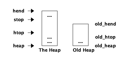
+high_water, old_hend, old_htop, old_heap,
gen_gcs, max_gen_gcs, off_heap,  mbuf, mbuf_sz, psd, bin_vheap_sz,
bin_vheap_mature, bin_old_vheap_sz, bin_old_vheap+.
12.5. Other interesting memory areas
12.5.1. The atom table.
TODO ==== Code TODO ==== Constants TODO
14. IO, Ports and Networking (10p)
Within Erlang, all communication is done by asynchronous signaling. The communication between an Erlang node and the outside world is done through a port. A port is an interface between Erlang processes and an external resource. In early versions of Erlang a port behaved very much in the same way as a process and you communicated by sending and receiving signals. You can still communicate with ports this way but there are also a number of BIFs to communicate directly with a port.
In this chapter we will look at how ports are used as a common interface for all IO, how ports communicate with the outside world and how Erlang processes communicate with ports. But first we will look at how standard IO works on a higher level.
14.1. Standard IO
-
IO protocol
-
group leader
-
erlang:display — a BIF that sends directly to node’s std out
-
io:format — sends through io protocol and the group leader
-
Redirecting standard IO at startup (detached mode)
-
Standard in and out
14.2. Ports
A port is the process like interface between Erlang processes and everything that is not Erlang processes. The programmer can to a large extent pretend that everything in the world behaves like an Erlang process and communicate through message passing.
Each port has an owner, more on this later, but all processes who know about the port can send messages to the port. In figure REF we see how a process can communicate with the port and how the port is communicating to the world outside the Erlang node.
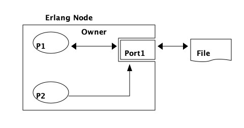
Process P1 has opened a port (Port1) to a file, and is the owner of the port and can receive messages from the port. Process P2 also has a handle to the port and can send messages to the port. The processes and the port reside in an Erlang node. The file lives in the file and operating system on the outside of the Erlang node.
If the port owner dies or is terminated the port is also killed. When a port terminates all external resources should also be cleaned up. This is true for all ports that come with Erlang and if you implement your own port you should make sure it does this cleanup.
14.2.1. Different types of Ports
There are three different classes of ports: file descriptors, external programs and drivers. A file descriptor port makes it possible for a process to access an already opened file descriptor. A port to an external program invokes the external program as a separate OS process. A driver port requires a driver to be loaded in the Erlang node.
All ports are created by a call to erlang:open_port(PortName, PortSettings).
A file descriptor port is opened with {fd, In, Out} as the PortName. This class of ports is used by some internal ERTS servers like the old shell. They are considered to not be very efficient and hence seldom used.
An external program port can be used to execute any program in the native OS of the Erlang node. To open an external program port you give either the argument {spawn, Command} or {spawn_executable, FileName} with the name of the external program. This is the easiest and one of the safest way to interact with code written in other programming languages. Since the external program is executed in its own OS process it will not bring down the Erlang node if it crashes. (It can of course use up all CPU or memory or do a number of other things to bring down the whole OS, but it is much safer than a linked in driver or a NIF).
A driver port requires that a driver program has been loaded with ERTS. Such a port is started with either {spawn, Command} or {spawn_driver, Command}. Writing your own linked in driver can be an efficient way to interface for example some C library code that you would like to use. Note that a linked in driver executes in the same OS process as the Erlang node and a crash in the driver will bring down the whole node. Details about how to write an Erlang driver in general can be found in Chapter 16.
Erlang/OTP comes with a number port drivers implementing the
predefined port types. There are the common drivers available on all
platforms: tcp_inet, udp_inet, sctp_inet, efile, zlib_drv,
ram_file_drv, binary_filer, tty_sl. These drivers are used to
implement e.g. file handling and sockets in Erlang. On Windows there
is also a driver to access the registry: registry_drv. And on most
platforms there are example drivers to use when implementing your own
driver like: multi_drv and sig_drv.

Ports to Linked in Drivers
Creating
Commands
Implementation
See chapter Chapter 16 for details of how to implement your own linked in driver.
II: 运行 ERTS
19. 调试
| This chapter is still a stub and it’s being heavily worked on. If planning a major addition to this chapter, please synchronize with the authors to avoid conflicts or duplicated efforts. You are still welcome to submit your feedback using a GitHub Issue. You can use the same mechanism to suggest sections that you believe should be included in this chapter, too. |
19.1. Preliminary Outline
-
Introduction
-
debugger
-
dbg
-
redbug
-
Crash dumps
-
…
19.2. Introduction
Debugging is the art of identifying and removing errors (i.e. bugs) from software. This section covers the most common Erlang debugging tools and techniques. Even if step-by-step debugging tools such as the Debugger exist in Erlang, the most effective debugging techniques in Erlang are the ones based on the so-called Erlang tracing facilities, which will be discussed in detail in chapter Chapter 18. This chapter also covers the concept of Crash Dump, a readable text file generated by the Erlang Runtime System when an unrecoverable error is detected, for example when the system runs out of memory or when an emulator limit is reached. Crash Dumps can are extremely precious for post-mortem analysis of Erlang nodes and you will learn how to read and interpret them.
19.3. debugger
TODO
19.4. dbg
TODO
19.5. Redbug
Redbug is a debugging utility which allows you to easily interact with the Erlang tracing facilities. It is an external library and therefore it has to be installed separately. One of the best Redbug features is its ability to shut itself down in case of overload.
19.5.1. Installing Redbug
You can clone redbug via:
$ git clone https://github.com/massemanet/redbugYou can then compile it with:
$ cd redbug
$ make
Ensure redbug is included in your path when starting an Erlang shell
and you are set to go. This can be done by explicitely adding the path
to the redbug beam files when invoking erl:
$ erl -pa /path/to/redbug/ebinAlternatively, the following line can be added to the ~/.erlang
file. This will ensure that the path to redbug gets included
automatically at every startup:
code:add_patha("/path/to/redbug/ebin").19.5.2. Using Redbug
Redbug is safe to be used in production, thanks to a self-protecting mechanism against overload, which kills the tool in case too many tracing messages are sent, preventing the Erlang node to become overloaded. Let’s see it in action:
$ erl
Erlang/OTP 19 [erts-8.2] [...]

Eshell V8.2 (abort with ^G)
1> l(redbug). (1)
{module,redbug}
2> redbug:start("lists:sort/1"). (2)
{30,1}
3> lists:sort([3,2,1]).
[1,2,3]

% 15:20:20 <0.31.0>({erlang,apply,2}) (3)
% lists:sort([3,2,1])
redbug done, timeout - 1 (4)| 1 | First, we ensure that the redbug module is available and loaded. |
| 2 | We then start redbug. We are interested in the function
named sort with arity 1, exported by the module lists.
Remember that, in Erlang lingo, the arity represents the number
of input arguments that a given function takes. |
| 3 | Finally, we invoke the lists:sort/1 function and we verify that
a message is produced by redbug. |
| 4 | After the default timeout (15 seconds) is reached, redbug stops and displays the message "redbug done". Redbug is also kind enough to tell us the reason why it stopped (timeout) and the number of messages that collected until that point (1). |
Let’s now look at the actual message produced by redbug. By default messages are printed to the standard output, but it’s also possible to dump them to file:
% 15:20:20 <0.31.0>({erlang,apply,2})
% lists:sort([3,2,1])
Depending on the version of redbug you are using, you may get a
slightly different message. In this case, the message is split across
two lines. The first line contains a timestamp, the Process Identifier
(or PID) of the Erlang process which invoked the function and the
caller function. The second line contains the function called,
including the input arguments. Both lines are prepended with a %,
which reminds us of the syntax for Erlang comments.
We can also ask Redbug to produce an extra message for the return value. This is achieved using the following syntax:
4> redbug:start("lists:sort/1->return").
{30,1}
Let’s invoke the lists:sort/1 function again. This time the output
from redbug is slightly different.
5> lists:sort([3,2,1]).
[1,2,3]

% 15:35:52 <0.31.0>({erlang,apply,2})
% lists:sort([3,2,1])

% 15:35:52 <0.31.0>({erlang,apply,2})
% lists:sort/1 -> [1,2,3]
redbug done, timeout - 1
In this case two messages are produced, one when entering the function and one when leaving the same function.
When dealing with real code, trace messages can be complex and therefore hardly readable. Let’s see what happens if we try to trace the sorting of a list containing 10.000 elements.
6> lists:sort(lists:seq(10000, 1, -1)).
[1,2,3,4,5,6,7,8,9,10,11,12,13,14,15,16,17,18,19,20,21,22,
23,24,25,26,27,28,29|...]

% 15:48:42.208 <0.77.0>({erlang,apply,2})
% lists:sort([10000,9999,9998,9997,9996,9995,9994,9993,9992,9991,9990,9989,9988,9987,9986,
% 9985,9984,9983,9982,9981,9980,9979,9978,9977,9976,9975,9974,9973,9972,9971,
% 9970,9969,9968,9967,9966,9965,9964,9963,9962,9961,9960,9959,9958,9957,9956,
% 9955,9954,9953,9952,9951,9950,9949,9948,9947,9946,9945,9944,9943,9942,9941,
% 9940,9939,9938,9937,9936,9935,9934,9933,9932,9931,9930,9929,9928,9927,9926,
% 9925,9924,9923,9922,9921,9920,9919,9918,9917,9916,9915,9914,9913,9912,9911,
% [...]
% 84,83,82,81,80,79,78,77,76,75,74,73,72,71,70,69,68,67,66,65,64,63,62,61,60,
% 59,58,57,56,55,54,53,52,51,50,49,48,47,46,45,44,43,42,41,40,39,38,37,36,35,
% 34,33,32,31,30,29,28,27,26,25,24,23,22,21,20,19,18,17,16,15,14,13,12,11,10,9,
% 8,7,6,5,4,3,2,1])

% 15:48:42.210 <0.77.0>({erlang,apply,2}) lists:sort/1 ->
% [1,2,3,4,5,6,7,8,9,10,11,12,13,14,15,16,17,18,19,20,21,22,
% 23,24,25,26,27,28,29,30,31,32,33,34,35,36,37,38,39,40,41,
% 42,43,44,45,46,47,48,49,50,51,52,53,54,55,56,57,58,59,60,
% 61,62,63,64,65,66,67,68,69,70,71,72,73,74,75,76,77,78,79,
% 80,81,82,83,84,85,86,87,88,89,90,91,92,93,94,95,96,97,98,
% 99,100,101,102,103,104,105,106,107,108,109,110,111,112,113,
% [...]
% 9951,9952,9953,9954,9955,9956,9957,9958,9959,9960,9961,
% 9962,9963,9964,9965,9966,9967,9968,9969,9970,9971,9972,
% 9973,9974,9975,9976,9977,9978,9979,9980,9981,9982,9983,
% 9984,9985,9986,9987,9988,9989,9990,9991,9992,9993,9994,
% 9995,9996,9997,9998,9999,10000]
redbug done, timeout - 1
Most of the output has been truncated here, but you should get the
idea. To improve things, we can use a couple of redbug options. The
option {arity, true} instructs redbug to only display the number of
input arguments for the given function, instead of their actual
value. The {print_return, false} option tells Redbug not to display
the return value of the function call, and to display a … symbol,
instead. Let’s see these options in action.
7> redbug:start("lists:sort/1->return", [{arity, true}, {print_return, false}]).
{30,1}

8> lists:sort(lists:seq(10000, 1, -1)).
[1,2,3,4,5,6,7,8,9,10,11,12,13,14,15,16,17,18,19,20,21,22,
23,24,25,26,27,28,29|...]

% 15:55:32 <0.77.0>({erlang,apply,2})
% lists:sort/1

% 15:55:32 <0.77.0>({erlang,apply,2})
% lists:sort/1 -> '...'
redbug done, timeout - 1
By default, redbug stops after 15 seconds or after 10 messages are
received. Those values are a safe default, but they are rarely
enough. You can bump those limits by using the time and msgs
options. time is expressed in milliseconds.
9> redbug:start("lists:sort/1->return", [{arity, true}, {print_return, false}, {time, 60 * 1000}, {msgs, 100}]).
{30,1}
We can also activate redbug for several function calls
simultaneously. Let’s enable tracing for both functions lists:sort/1
and lists:sort_1/3 (an internal function used by the former):
10> redbug:start(["lists:sort/1->return", "lists:sort_1/3->return"]).
{30,2}

11> lists:sort([4,4,2,1]).
[1,2,4,4]

% 18:39:26 <0.32.0>({erlang,apply,2})
% lists:sort([4,4,2,1])

% 18:39:26 <0.32.0>({erlang,apply,2})
% lists:sort_1(4, [2,1], [4])

% 18:39:26 <0.32.0>({erlang,apply,2})
% lists:sort_1/3 -> [1,2,4,4]

% 18:39:26 <0.32.0>({erlang,apply,2})
% lists:sort/1 -> [1,2,4,4]
redbug done, timeout - 2
Last but not least, redbug offers the ability to only display results for matching input arguments. This is when the syntax looks a bit like magic.
12> redbug:start(["lists:sort([1,2,5])->return"]).
{30,1}

13> lists:sort([4,4,2,1]).
[1,2,4,4]

14> lists:sort([1,2,5]).
[1,2,5]

% 18:45:27 <0.32.0>({erlang,apply,2})
% lists:sort([1,2,5])

% 18:45:27 <0.32.0>({erlang,apply,2})
% lists:sort/1 -> [1,2,5]
redbug done, timeout - 1
In the above example, we are telling redbug that we are only
interested in function calls to the lists:sort/1 function when the
input arguments is the list [1,2,5]. This allows us to remove a huge
amount of noise in the case our target function is used by many actors
at the same time and we are only interested in a specific use case.
Oh, and don’t forget that you can use the underscore as a wildcard:
15> redbug:start(["lists:sort([1,_,5])->return"]).  {30,1}

16> lists:sort([1,2,5]).  [1,2,5]

% 18:49:07 <0.32.0>({erlang,apply,2}) lists:sort([1,2,5])

% 18:49:07 <0.32.0>({erlang,apply,2}) lists:sort/1 -> [1,2,5]

17> lists:sort([1,4,5]).  [1,4,5]

% 18:49:09 <0.32.0>({erlang,apply,2}) lists:sort([1,4,5])

% 18:49:09 <0.32.0>({erlang,apply,2}) lists:sort/1 -> [1,4,5] redbug
% done, timeout - 2
This section does not pretend to be a comprehensive guide to redbug, but it should be enough to get you going. To get a full list of the available options for redbug, you can ask the tool itself:
18> redbug:help().19.6. Crash Dumps
TODO
20. 运维
One guiding principle behind the design of the runtime system is that bugs are more or less inevitable. Even if through an enormous effort you manage to build a bug free application you will soon learn that the world or your user changes and your application will need to be "fixed."
The Erlang runtime system is designed to facilitate change and to minimize the impact of bugs.
The impact of bugs is minimized by compartmentalization. This is done from the lowest level where each data structure is separate and immutable to the highest level where running systems are dived into separate nodes. Change is facilitated by making it easy to upgrade code and interacting and examining a running system.
20.1. Connecting to the System
We will look at many different ways to monitor and maintain a running system. There are many tools and techniques available but we must not forget the most basic tool, the shell and the ability to connect a shell to node.
In order to connect two nodes they need to share or
know a secret pass phrase, called a cookie. As long
as you are running both nodes on the same machine
and the same user starts them they will automatically
share the cookie (in the file $HOME/.erlang.cookie).
We can see this in action by starting two nodes, one Erlang node
and one Elixir node. First we start an Erlang node called
node1.
$ erl -sname node1
Erlang/OTP 19 [erts-8.1] [source-0567896] [64-bit] [smp:4:4]
              [async-threads:10] [hipe] [kernel-poll:false]

Eshell V8.1  (abort with ^G)
(node1@GDC08)1> nodes().
[]
(node1@GDC08)2>
Then we start an Elixir node called node2:
$ iex --sname node2
Erlang/OTP 19 [erts-8.1] [source-0567896] [64-bit] [smp:4:4]
              [async-threads:10] [hipe] [kernel-poll:false]

Interactive Elixir (1.4.0) - press Ctrl+C to exit (type h() ENTER for help)
iex(node2@GDC08)1>
In Elixir we can connect the nodes by running the command Node.connect
name. In Erlang you do this with net_kernel:connect(Name).
The node connection is bidirectional so you only
need to run the command on one of the nodes.
iex(node2@GDC08)1> Node.connect :node1@GDC08
true
iex(node2@GDC08)2>
In the distributed case this is somewhat more complicated since we
need to make sure that all nodes know or share the cookie. This can
be done in three ways. You can set the cookie used when talking to a
specific node, you can set the same cookie for all systems at start up
with the -set_cookie parameter, or you can copy the file
.erlang.cookie to the home directory of the user running the system
on each machine.
The last alternative, to have the same cookie in the cookie file of each machine in the system is usually the best option since it makes it easy to connect to the nodes from a local OS shell. Just set up some secure way of logging in to the machine either through VPN or ssh. In the next section we will see how to then connect a shell to a running node.
Using the second option it might look like this:
happi@GDC08:~$ cat ~/.erlang.cookie
pepparkaka
happi@GDC08:~$ ssh gds01

happi@gds01:~$ erl -sname node3 -setcookie pepparkaka
Erlang/OTP 18 [erts-7.3] [source-d2a6d81] [64-bit] [smp:8:8]
              [async-threads:10] [hipe] [kernel-poll:false]

Eshell V7.3  (abort with ^G)
(node3@gds01)1> net_kernel:connect('node1@GDC08').
true
(node3@gds01)2> nodes().
[node1@GDC08,node2@GDC08]
(node3@gds01)3>
A Potential Problem with Different Cookies
Note that the default for the Erlang distribution is to create a
fully connected network. That is, all nodes are connected to all
other nodes in the network. In the example, once node3 connects to
node1 it also is connected to node2.
If each node has its own cookie you will have to tell each node the
cookies of each other node before you try to connect them. You can
start up a node with the flag -connect_all false in order to
prevent the system from trying to make a fully connected network.
Alternatively, you can start a node as hidden with the flag
-hidden, which makes node connections to that node non transitive.
|
Now that we know how to connect nodes, even on different machines, to each other, we can look at how to connect a shell to a node.
20.2. The Shell
The Elixir and the Erlang shells works much the same way as a shell or a terminal window on your computer, except that they give you a terminal window directly into your runtime system. This gives you an extremely powerful tool, a basically CLI with full access to the runtime. This is fantastic for operation and maintenance.
In this section we will look at different ways of connecting to a node through the shell and some of the shell’s perhaps less known but more powerful features.
20.2.1. Configuring Your Shell
Both the Elixir shell and the Erlang shell can be configured to provide you with shortcuts for functions that you often use.
The Elixir shell will look for the file .iex.exs first in
the local directory and then in the users home directory.
The code in this file is executed in the shell process
and all variable bindings will be available in the shell.
In this file you can configure aspects such as the syntax coloring and the size of the history. [See hexdocs for a full documentation.](https://hexdocs.pm/iex/IEx.html#module-the-iex-exs-file)
You can also execute arbitrary code in the shell context.
When the Erlang runtime system starts, it first interprets the
code in the Erlang configuration file. The default location
of this file is in the users home directory ~/.erlang.
This file is usually used to load the user default settings for the shell by adding the line
code:load_abs("/home/happi/.config/erlang/user_default").
Replace "/home/happi/.config/erlang/" with the absolute path you want to use.
If you call a local function from the shell it will try to
call this function first in the module user_default and
then in the module shell_default (located in stdlib).
This is how command such as ls() and help() are implemented.
20.2.2. Connecting a Shell to a Node
When running a production system you will want to start the nodes in
daemon mode through run_erl. We will go through how to start a node
and some of the best practices for deployment and running in
production in [xxx](#ch.live). Fortunately, even when you have started
a system in daemon mode, without a shell, you can connect a shell to
the system. There are actually several ways to do that. Most of these
methods rely on the normal distribution mechnaisms and hence require
that you have the same Erlang cookie on both machines as described
in the previous section.
Remote shell (Remsh)
The easiest and probably the most common way to connect to an Erlang
node is by starting a named node that connects to the system node
through a remote shell. This is done with the erl command line flag
-remsh Name. Note that you need to start a named node in order to
be able to connect to another node, so you also need the -name or
-sname flag. Also, note that these are arguments to the Erlang
runtime so if you are starting an Elixir shell you need to add an
extra - to the flags, like this:
$ iex --sname node4 --remsh node2@GDC08
Erlang/OTP 19 [erts-8.1] [source-0567896] [64-bit] [smp:4:4]
              [async-threads:10] [hipe] [kernel-poll:false]

Interactive Elixir (1.4.0) - press Ctrl+C to exit (type h() ENTER for help)
iex(node2@GDC08)1>
Another thing to note here is that in order to start a remote Elixir shell you need to have IEx running on that node. There is no problem to connect Elixr and Erlang nodes to each other as we saw in the previous section, but you need to have the code of the shell you want to run loaded on the node you connect to.
It is also worth noting that there is no security built into either
the normal Erlang distribution or to the remote shell implementation.
You do not want to have your system node exposed to the internet and
you do not want to connect from your local machine to a node. The safest
way is probably to have a VPN tunnel to your live environment and use ssh
to connect a machine running one of your live nodes. Then you can connect
to one of the nodes using remsh.
It is important to understand that there are actually two nodes
involved when you start a remote shell. The local node, named node4
in the previous example and the remote node node2. These nodes can
be on the same machine or on different machines. The local node is
always running on the machine on which you gave the iex or erl
command. On the local node there is a process running the tty
program which interacts with the terminal window. The actual shell
process runs on the remote node. This means, first of all, that the
code for the shell you want to run (i.e. iex or the Erlang shell) has
to exist at the remote node. It also means that code is executed on
the remote node. And it also means that any shell default settings are
taken from the settings of the remote machine.
Imagine that we have the following .erlang file in our home directory
on the machine GDC08.
code:load_abs("/home/happi/.config/erlang/user_default").
io:format("ERTS is starting in sn",[os:cmd("pwd")]).
And the <filename>user_default.erl</filename> file looks like this:
-module(user_default).
-export([tt/0]).
tt() → test.
Then we create two directories ~/example/dir1 and ~/example/dir2
and we put two different .iex.exs files in those directories.
IO.puts "iEx starting in " pwd() IO.puts "iEx starting on " IO.puts Node.self
IEx.configure( colors: [enabled: true], alive_prompt: [ "\e[G", "(%node)", "%prefix", "<d1>", ] |> IO.ANSI.format |> IO.chardata_to_string )
IO.puts "iEx starting in " pwd() IO.puts "iEx starting on " IO.puts Node.self
IEx.configure( colors: [enabled: true], alive_prompt: [ "\e[G", "(%node)", "%prefix", "<d2>", ] |> IO.ANSI.format |> IO.chardata_to_string )
Now if we start four different nodes from these directories we will see how the shell configurations are loaded.
GDC08:~/example/dir1$ iex --sname node1
Erlang/OTP 19 [erts-8.1] [source-0567896] [64-bit]
              [smp:4:4] [async-threads:10] [hipe] [kernel-poll:false]

ERTS is starting in /home/happi/example/dir1
 on [node1@GDC08]
Interactive Elixir (1.4.0) - press Ctrl+C to exit (type h() ENTER for help)
iEx starting in
/home/happi/example/dir1
iEx starting on
node1@GDC08
(node1@GDC08)iex<d1>GDC08:~/example/dir2$ iex --sname node2
Erlang/OTP 19 [erts-8.1] [source-0567896] [64-bit]
[smp:4:4] [async-threads:10] [hipe] [kernel-poll:false]
ERTS is starting in /home/happi/example/dir2
on [node2@GDC08]
Interactive Elixir (1.4.0) - press Ctrl+C to exit (type h() ENTER for help)
iEx starting in
/home/happi/example/dir2
iEx starting on
node2@GDC08
(node2@GDC08)iex<d2>GDC08:~/example/dir1$ iex --sname node3 --remsh node2@GDC08
Erlang/OTP 19 [erts-8.1] [source-0567896] [64-bit] [smp:4:4]
[async-threads:10] [hipe] [kernel-poll:false]
ERTS is starting in /home/happi/example/dir1
on [node3@GDC08]
Interactive Elixir (1.4.0) - press Ctrl+C to exit (type h() ENTER for help)
iEx starting in
/home/happi/example/dir2
iEx starting on
node2@GDC08
(node2@GDC08)iex<d2>GDC08:~/example/dir2$ erl -sname node4
Erlang/OTP 19 [erts-8.1] [source-0567896] [64-bit] [smp:4:4]
[async-threads:10] [hipe] [kernel-poll:false]
ERTS is starting in /home/happi/example/dir2
on [node4@GDC08]
Eshell V8.1 (abort with ^G)
(node4@GDC08)1> tt().
test
(node4@GDC08)2>The shell configuration is loaded from the node running the shell, as you can see from the previous examples. If we were to connect to a node on a different machine, these configurations would not be present.
You can actually change which node and shell you are connected to by going into job control mode.
Job Control Mode
By pressing control+G (ctrl-G) you enter the job control mode (JCL). You are then greeted by another prompt:
User switch command
 -->
By typing h (followed by enter)
you get a help text with the available commands in JCL:
  c [nn]            - connect to job
  i [nn]            - interrupt job
  k [nn]            - kill job
  j                 - list all jobs
  s [shell]         - start local shell
  r [node [shell]]  - start remote shell
  q                 - quit erlang
  ? | h             - this message
The interesting command here is the r command which
starts a remote shell. You can give it the name of the
shell you want to run, which is needed if you want to start
an Elixir shell, since the default is the standard Erlang shell.
Once you have started a new job (i.e. a new shell)
you need to connect to that job with the c command.
You can also list all jobs with j.
(node2@GDC08)iex<d2>
User switch command
 --> r node1@GDC08 'Elixir.IEx'
 --> c
Interactive Elixir (1.4.0) - press Ctrl+C to exit (type h() ENTER for help)
iEx starting in
/home/happi/example/dir1
iEx starting on
node1@GDC08
See the [Erlang Shell manual](http://erlang.org/doc/man/shell.html) for a full description of JCL mode.
You can quit your session by typing ctrl+G q [enter]. This
shuts down the local node. You do not want to quit with
any of q()., halt(), init:stop(), or System.halt.
All of these will bring down the remote node which seldom
is what you want when you have connected to a live server.
Instead use ctrl+\, ctrl+c ctrl+c, ctrl+g q [enter]
or ctrl+c a [enter].
If you do not want to use a remote shell, which requires you to have two instances of the Erlang runtime system running, there are actually two other ways to connect to a node. You can also connect either through a Unix pipe or directly through ssh, but both of these methods require that you have prepared the node you want to connect to by starting it in a special way or by starting an ssh server.
Connecting through a Pipe
By starting the node through the command run_erl you will
get a named pipe for IO and you can attach a shell to that
pipe without the need to start a whole new node. As we shall
see in the next chapter there are some advantages to using
run_erl instead of just starting Erlang in daemon mode,
such as not losing standard IO and standard error output.
The run_erl command is only available on Unix-like operating systems that implement pipes. If you start your system with run_erl, something like:
> run_erl -daemon log/erl_pipe log "erl -sname node1"or
> run_erl -daemon log/iex_pipe log "iex --sname node2"You can then attach to the system through the named pipe (the first argument to run_erl).
> to_erl dir1/iex_pipe

iex(node2@GDC08)1>
You can exit the shell by sending EOF (ctrl+d) and leave the system
running in the background. Note that with to_erl the terminal is
connected directly to the live node so if you exit with ctrl-G q
[enter] you will bring down that node, probably not what you want.
The last method for connecting to the node is through ssh.
Connecting through SSH
Erlang comes with a built in ssh server which you can start on your node and then connect to directly. The [documentation for the ssh module](http://erlang.org/doc/man/ssh.html) explains all the details. For a quick test all you need is a server key which you can generate with ssh-keygen:
> mkdir ~/ssh-test/
> ssh-keygen -t rsa -f ~/ssh-test/ssh_host_rsa_key
Then you start the ssh daemon on the Erlang node:
gds01> erl
Erlang/OTP 18 [erts-7.3] [source-d2a6d81] [64-bit] [smp:8:8]
              [async-threads:10] [hipe] [kernel-poll:false]

Eshell V7.3  (abort with ^G)
1> ssh:start().
{ok,<0.47.0>}
2> ssh:daemon(8021, [{system_dir, "/home/happi/.ssh/ehost/"},
                     {auth_methods, "password"},
                     {password, "pwd"}]).
You can now connect from another machine:
happi@GDC08:~> ssh -p 8021 happi@gds01
happi@gds01's password: [pwd]
Eshell V7.3  (abort with ^G)
1>
In a real world setting you would want to set up your server and user ssh keys as described in the documentation. At least you would want to have a better password.
To disconnect from the shell you need to shut down your terminal
window. Using q() or init:stop() would bring down the node.
In this shell you do not have access to neither JCL mode (ctrl+g)
nor the BREAK mode (ctrl+c).
The break mode is really powerful when developing, profiling and debugging. We will take a look at it next.
20.2.3. Breaking (out or in).
When you press ctrl+c you enter BREAK mode. This is most
often used just to break out of the shell by either tying
a [enter] for abort or by hitting ctrl+c once more.
But you can actually use this mode to break in to the
internals of the Erlang runtime system.
When you enter BREAK mode you get a short menu:
BREAK: (a)bort (c)ontinue (p)roc info (i)nfo (l)oaded
       (v)ersion (k)ill (D)b-tables (d)istribution
Abort exits the node and continue takes you back in to
the shell. Hitting p [enter] will give you internal
information about all processes in the system. We
will look closer at what this information means
in the next chapter (See [xxx](#ch.processes)).
You can also get information about the memory and
the memory allocators in the node through the
info choice (i [enter]). In [xxx](#ch.memory)
we will look at how to decipher this information.
You can see all loaded modules and their sizes with
l [enter] and the system version with v [enter],
while k [enter] will let you step through all processes
and inspect them and kill them. Capital D [enter] will
show you information about all the ETS tables in the
system and lower case d [enter] will show you
information about the distribution. That is basically
just the node name.
If you have built your runtime with OPPROF or DEBUG you will be able to get even more information. We will look at how to do this in Appendix A. The code for the break mode can be found in <filename>[OTP_SOURCE]/erts/emulator/beam/break.c</filename>.
Note that going into break mode freezes the node. This is not something you want to do on a production system. But when debugging or profiling in a test system, this mode can help us find bugs and bottlenecks, as we will see later in this book.
Appendix A: 构造 Erlang 运行时系统
In this chapter we will look at different way to configure and build Erlang/OTP to suite your needs. We will use an Ubuntu Linux for most of the examples. If you are using a different OS you can find detailed instructions on how to build for that OS in the documentation in the source code (in HOWTO/INSTALL.md), or on the web INSTALL.html.
There are basically two ways to build the runtime system, the traditional way with autoconf, configure and make or with the help of kerl.
I recommend that you first give the traditional way a try, that way you will get a better understanding of what happens when you build and what settings you can change. Then go over to using kerl for your day to day job of managing configurations and builds.
A.1. First Time Build
To get you started we will go though a step by step process of building the system from scratch and then we will look at how you can configure your system for different purposes.
This step by step guide assumes that you have a modern Ubuntu installation. We will look at how to build on OS X and Windows later in this chapter.
A.1.1. Prerequisites
You will need a number of tools in order to fetch, unpack and build from source. The file Install.md lists some of the most important ones.
Gven that we have a recent Ubuntu installation to start with many of the needed tools such as tar, make, perl and gcc should already be installed. But some tools like git, m4 and ncurses will probably need to be installed.
If you add a source URI to your apt configuration you will be able to use the build-dep command to get the needed sources to build erlang. You can do this by uncommenting the deb-src line for your distribution in /etc/apt/sources.list.
For the Yakkety Yak release you could add the line by:
> sudo cat "deb-src http://se.archive.ubuntu.com/ubuntu/ \
yakkety main restricted" >> /etc/apt/sources.list
Then the following commands will get almost all the tools you need:
> sudo apt-get install git autoconf m4
> sudo apt-get build-dep erlang
If you have a slightly older version of Ubuntu like Saucy and you want to build with wx support, you need to get the wx libraries:
> sudo apt-key adv --fetch-keys http://repos.codelite.org/CodeLite.asc
> sudo apt-add-repository 'deb http://repos.codelite.org/wx3.0/ubuntu/ saucy universe'
> sudo apt-get update
> sudo apt-get install libwxbase3.0-0-unofficial libwxbase3.0-dev libwxgtk3.0-0-unofficial \
libwxgtk3.0-dev wx3.0-headers wx-common libwxbase3.0-dbg libwxgtk3.0-dbg wx3.0-i18n \
wx3.0-examples wx3.0-doc
You might also want to create a directory where you keep the source code and also install your home built version without interfering with any pre built and system wide installations.
> cd
> mkdir otp
A.2. Getting the source
There are two main ways of getting the source. You can download a tarball from erlang.org or you can check out the source code directly from Github.
If you want to quickly download a stable version of the source try:
> cd ~/otp
> wget http://erlang.org/download/otp_src_19.1.tar.gz
> tar -xzf otp_src_19.1.tar.gz
> cd otp_src_19.1
> export ERL_TOP=`pwd`
or if you want to be able to easilly update to the latest bleeding edge or you want to contribute fixes back to the comunity you can check out the source through git:
> cd ~/otp
> git clone https://github.com/erlang/otp.git source
> cd source
> export ERL_TOP=`pwd`
> ./otp_build autoconf
Now you are ready to build and install Erlang:
> export LANG=C
> ./configure --prefix=$HOME/otp/install
> make
> make install
> export PATH=$HOME/otp/install/bin/:$PATH
> export ROOTDIR=$HOME/otp/install/
A.3. Building with Kerl
An easier way to build especially if you want to have several different builds available to experiment with is to build with Kerl.
Appendix B: BEAM 指令
Here we will go through most of the instructions in the BEAM generic instruction set in detail. In the next section we list all instructions with a brief explanation generated from the documentaion in the code (see lib/compiler/src/genop.tab).
B.1. Functions and Labels
B.1.1. label Lbl
Instruction number 1 in the generic instruction set is not really an instruction at all. It is just a module local label giving a name, or actually a number to the current position in the code.
Each label potentially marks the beginning of a basic block since it is a potential destination of a jump.
B.1.2. func_info Module Function Arity
The code for each function starts with a func_info instruction. This instruction is used for generating a function clause error, and the execution of the code in the function actually starts at the label following the func_info instruction.
Imagine a function with a guard:
id(I) when is_integer(I) -> I.The Beam code for this function might look like:
{function, id, 1, 4}.
  {label,3}.
    {func_info,{atom,test1},{atom,id},1}.
  {label,4}.
    {test,is_integer,{f,3},[{x,0}]}.
    return.
Here the meta information {function, id, 1, 4} tells us that execution of the id/1 function will start at label 4. At label 4 we do an is_integer on x0 and if we fail we jump to label 3 (f3) which points to the func_info instruction, which will generate a function clause exception. Otherwise we just fall through and return the argument (x0).
Function info instruction points to an Export record (defined in erts/emulator/beam/export.h) and located somewhere else in memory. The few dedicated words of memory inside that record are used by the tracing mechanism to place a special trace instruction which will trigger for each entry/return from the function by all processes.
|
B.2. Test instructions
B.2.1. Type tests
The type test instructions (is_\* Lbl Argument) checks whether the argument is of the given type and if not jumps to the label Lbl. The beam disassembler wraps all these instructions in a test instruction. E.g.:
{test,is_integer,{f,3},[{x,0}]}.The current type test instructions are is_integer, is_float, is_number, is_atom, is_pid, is_reference, is_port, is_nil, is_binary, is_list, is_nonempty_list, is_function, is_function2, is_boolean, is_bitstr, and is_tuple.
And then there is also one type test instruction of Arity 3: test_arity Lbl Arg Arity. This instruction tests that the arity of the argument (assumed to be a tuple) is of Arity. This instruction is usually preceded by an is_tuple instruction.
B.2.2. Comparisons
The comparison instructions (is_\* Lbl Arg1 Arg2) compares the two arguments according to the instructions and jumps to Lbl if the comparison fails.
The comparison instructions are: is_lt, is_ge, is_eq, is_ne, is_eq_exact, and is_ne_exact.
Remember that all Erlang terms are ordered so these instructions can compare any two terms. You can for example test if the atom self is less than the pid returned by self(). (It is.)
Note that for numbers the comparison is done on the Erlang type number, see Chapter 4. That is, for a mixed float and integer comparison the number of lower precision is converted to the other type before comparison. For example on my system 1 and 1.0 compares as equal, as well as 9999999999999999 and 1.0e16. Comparing floating point numbers is always risk and best avoided, the result may wary depending on the underlying hardware.
If you want to make sure that the integer 1 and the floating point number 1.0 are compared different you can use is_eq_exact and is_ne_exact. This corresponds to the Erlang operators =:= and =/=.
B.3. Function Calls
In this chapter we will summarize what the different call instructions does. For a thorough description of how function calls work see Chapter 8.
B.3.1. call Arity Label
Does a call to the function of arity Arity in the same module at label Label. First count down the reductions and if needed do a context switch. Current code address after the call is saved into CP.
For all local calls the label is the second label of the function where the code starts. It is assumed that the preceding instruction at that label is func_info in order to get the MFA if a context switch is needed.
B.3.2. call_only Arity Label
Do a tail recursive call the function of arity Arity in the same module at label Label. First count down the reductions and if needed do a context switch. The CP is not updated with the return address.
B.3.3. call_last Arity Label Deallocate
Deallocate Deallocate words of stack, then do a tail recursive call to the function of arity Arity in the same module at label Label First count down the reductions and if needed do a context switch. The CP is not updated with the return address.
B.3.4. call_ext Arity Destination
Does an external call to the function of arity Arity given by Destination. Destination in assembly is usually written as {extfunc, Module, Function, Arity}, this is then added to imports section of the module. First count down the reductions and if needed do a context switch. CP will be updated with the return address.
B.3.5. call_ext_only Arity Destination
Does a tail recursive external call to the function of arity Arity given by Destination. Destination in assembly is usually written as {extfunc, Module, Function, Arity}. First count down the reductions and if needed do a context switch. The CP is not updated with the return address.
B.3.6. call_ext_last Arity Destination Deallocate
Deallocate Deallocate words of stack, then do a tail recursive external call to the function of arity Arity given by Destination. Destination in assembly is usually written as {extfunc, Module, Function, Arity}. First count down the reductions and if needed do a context switch. The CP is not updated with the return address.
B.3.7. bif0 Bif Reg, bif[1,2] Lbl Bif [Arg,…] Reg
Call the bif Bif with the given arguments, and store the result in Reg. If the bif fails, jump to Lbl. Zero arity bif cannot fail and thus bif0 doesn’t take a fail label.
Bif called by these instructions may not allocate on the heap nor trigger a garbage collection. Otherwise see: gc_bif.
|
B.3.8. gc_bif[1-3] Lbl Live Bif [Arg, …] Reg
Call the bif Bif with the given arguments, and store the result in Reg. If the bif fails, jump to Lbl. Arguments will be stored in x(Live), x(Live+1) and x(Live+2).
Because this instruction has argument Live, it gives us enough information to be able to trigger the garbage collection.
|
B.3.9. call_fun Arity
The instruction call_fun assumes that the arguments are placed in the first Arity argument registers and that the fun (the pointer to the closure) is placed in the register following the last argument x[Arity+1].
That is, for a zero arity call, the closure is placed in x[0]. For a arity 1 call x[0] contains the argument and x[1] contains the closure and so on.
Raises badarity if the arity doesn’t match the function object. Raises badfun if a non-function is passed.
|
B.3.10. apply Arity
Applies function call with Arity arguments stored in X registers. The module atom is stored in x[Arity] and the function atom is stored in x[Arity+1]. Module can also be represented by a tuple.
B.3.11. apply_last Arity Dealloc
Deallocates Dealloc elements on stack by popping CP, freeing the elements and pushing CP again. Then performs a tail-recursive call with Arity arguments stored in X registers, by jumping to the new location. The module and function atoms are stored in x[Arity] and x[Arity+1]. Module can also be represented by a tuple.
B.4. Stack (and Heap) Management
The stack and the heap of an Erlang process on Beam share the same memory area see Chapter 3 and Chapter 12 for a full discussion. The stack grows toward lower addresses and the heap toward higher addresses. Beam will do a garbage collection if more space than what is available is needed on either the stack or the heap.
These instructions are also used by non leaf functions for setting up and tearing down the stack frame for the current instruction. That is, on entry to the function the continuation pointer (CP) is saved on the stack, and on exit it is read back from the stack.
A function skeleton for a leaf function looks like this:
{function, Name, Arity, StartLabel}.
  {label,L1}.
    {func_info,{atom,Module},{atom,Name},Arity}.
  {label,L2}.
    ...
    return.
A function skeleton for a non leaf function looks like this:
{function, Name, Arity, StartLabel}.
  {label,L1}.
    {func_info,{atom,Module},{atom,Name},Arity}.
  {label,L2}.
    {allocate,Need,Live}.

    ...
    call ...
    ...

    {deallocate,Need}.
    return.
B.4.1. allocate StackNeed Live
Save the continuation pointer (CP) and allocate space for StackNeed extra words on the stack. If during allocation we run out of memory, call the GC and then first Live x registers will form a part of the root set. E.g. if Live is 2 then GC will save registers X0 and X1, rest are unused and will be freed.
When allocating on the stack, the stack pointer (E) is decreased.
       Before           After
         | xxx |            | xxx |
    E -> | xxx |            | xxx |
         |     |            | ??? | caller save slot
           ...         E -> | CP  |
           ...                ...
 HTOP -> |     |    HTOP -> |     |
         | xxx |            | xxx |
B.4.2. allocate_heap StackNeed HeapNeed Live
Save the continuation pointer (CP) and allocate space for StackNeed extra words on the stack. Ensure that there also is space for HeapNeed words on the heap. If during allocation we run out of memory, call the GC with Live amount of X registers to preserve.
| The heap pointer (HTOP) is not changed until the actual heap allocation takes place. |
B.4.3. allocate_zero StackNeed Live
This instruction works the same way as allocate, but it also clears
out the allocated stack slots with NIL.
       Before           After
         | xxx |            | xxx |
    E -> | xxx |            | xxx |
         |     |            | NIL | caller save slot
           ...         E -> | CP  |
           ...                ...
 HTOP -> |     |    HTOP -> |     |
         | xxx |            | xxx |
B.4.4. allocate_heap_zero StackNeed HeapNeed Live
The allocate_heap_zero instruction works as the allocate_heap instruction, but it also clears out the allocated stack slots with NIL.
B.4.5. test_heap HeapNeed Live
The test_heap instruction ensures there is space for HeapNeed words on the heap. If during allocation we run out of memory, call the GC with Live amount of X registers to preserve.
B.4.6. init N
The init instruction clears N stack words above the CP pointer by writing NIL to them.
B.4.7. deallocate N
The deallocate instruction is the opposite of the allocate. It restores the CP (continuation pointer) and deallocates N+1 stack words.
B.4.8. return
The return instructions jumps to the address in the continuation pointer (CP). The value of CP is set to 0 in C.
B.4.9. trim N Remaining
Pops the CP into a temporary variable, frees N words of stack, and places the CP back onto the top of the stack. (The argument Remaining is to the best of my knowledge unused.)
       Before           After
         | ??? |            | ??? |
         | xxx |       E -> | CP  |
         | xxx |            | ... |
    E -> | CP  |            | ... |
         |     |            | ... |
           ...                ...
 HTOP -> |     |    HTOP -> |     |
         | xxx |            | xxx |
B.5. Moving, extracting, modifying data
B.5.1. move Source Destination
Moves the value of the source Source (this can be a literal or a register) to the destination register Destination.
B.5.2. get_list Source Head Tail
This is a deconstruct operation for a list cell. Get the head and tail (or car and cdr) parts of a list (a cons cell), specified by Source and place them into the registers Head and Tail.
B.5.3. get_tuple_element Source Element Destination
This is an array indexed read operation. Get element with position Element from the Source tuple and place it into the Destination register.
B.5.4. set_tuple_element NewElement Tuple Position
This is a destructive array indexed update operation. Update the element of the Tuple at Position with the new NewElement.
B.6. Building terms.
B.6.1. put_list Head Tail Destination
Constructs a new list (cons) cell on the heap (2 words) and places its address into the Destination register. First element of list cell is set to the value of Head, second element is set to the value of Tail.
B.6.2. put_tuple Size Destination
Constructs an empty tuple on the heap (Size+1 words) and places its address into the Destination register. No elements are set at this moment. Put_tuple instruction is always followed by multiple put instructions which destructively set its elements one by one.
B.6.3. put Value
Places destructively a Value into the next element of a tuple, which was created by a preceding put_tuple instruction. Write address is maintained and incremented internally by the VM. Multiple put instructions are used to set contents for any new tuple.
B.6.4. make_fun2 LambdaIndex
Creates a function object defined by an index in the Lambda table of the module. A lambda table defines the entry point (a label or export entry), arity and how many frozen variables to take. Frozen variable values are copied from the current execution context (X registers) and stored into the function object.
B.7. Binary Syntax
B.7.5. bs_init2/6
TODO
B.7.6. bs_add/5
TODO
B.7.13. bs_save2/2
TODO
B.7.19. bs_append/8
TODO
B.8. Floating Point Arithmetic
B.8.1. fclearerror/0
TODO
B.8.2. fcheckerror/1
TODO
B.8.3. fmove/2
TODO
B.8.4. fconv/2
TODO
B.8.5. fadd/4
TODO
B.8.6. fsub/4
TODO
B.8.7. fmul/4
TODO
B.8.8. fdiv/4
TODO
B.8.9. fnegate/3
TODO
B.10. Exception handling
B.10.1. catch/2
TODO
B.10.2. catch_end/1
TODO
B.10.3. badmatch/1
TODO
B.10.4. if_end/0
TODO
B.10.5. case_end/1
TODO
B.12. Generic Instructions
| Name | Arity | Op Code | Spec | Documentation |
|---|---|---|---|---|
allocate |
2 |
12 |
allocate StackNeed, Live |
Allocate space for StackNeed words on the stack. If a GC is needed during allocation there are Live number of live X registers. Also save the continuation pointer (CP) on the stack. |
allocate_heap |
3 |
13 |
allocate_heap StackNeed, HeapNeed, Live |
Allocate space for StackNeed words on the stack and ensure there is space for HeapNeed words on the heap. If a GC is needed save Live number of X registers. Also save the continuation pointer (CP) on the stack. |
allocate_heap_zero |
3 |
15 |
allocate_heap_zero StackNeed, HeapNeed, Live |
Allocate space for StackNeed words on the stack and HeapNeed words on the heap. If a GC is needed during allocation there are Live number of live X registers. Clear the new stack words. (By writing NIL.) Also save the continuation pointer (CP) on the stack. |
allocate_zero |
2 |
14 |
allocate_zero StackNeed, Live |
Allocate space for StackNeed words on the stack. If a GC is needed during allocation there are Live number of live X registers. Clear the new stack words. (By writing NIL.) Also save the continuation pointer (CP) on the stack. |
apply |
1 |
112 |
||
apply_last |
2 |
113 |
||
badmatch |
1 |
72 |
||
bif0 |
2 |
9 |
bif0 Bif, Reg |
Call the bif Bif and store the result in Reg. |
bif1 |
4 |
10 |
bif1 Lbl, Bif, Arg, Reg |
Call the bif Bif with the argument Arg, and store the result in Reg. On failure jump to Lbl. |
bif2 |
5 |
11 |
bif2 Lbl, Bif, Arg1, Arg2, Reg |
Call the bif Bif with the arguments Arg1 and Arg2, and store the result in Reg. On failure jump to Lbl. |
bs_add |
5 |
111 |
||
bs_append |
8 |
134 |
||
bs_bits_to_bytes |
3 |
(110) |
DEPRECATED |
|
bs_bits_to_bytes2 |
2 |
(127) |
DEPRECATED |
|
bs_context_to_binary |
1 |
130 |
||
bs_final |
2 |
(88) |
DEPRECATED |
|
bs_final2 |
2 |
(126) |
DEPRECATED |
|
bs_get_binary |
5 |
(82) |
DEPRECATED |
|
bs_get_binary2 |
7 |
119 |
||
bs_get_float |
5 |
(81) |
DEPRECATED |
|
bs_get_float2 |
7 |
118 |
||
bs_get_integer |
5 |
(80) |
DEPRECATED |
|
bs_get_integer2 |
7 |
117 |
||
bs_get_position |
3 |
167 |
bs_get_position Ctx, Dst, Live |
Sets Dst to the current position of Ctx |
bs_get_tail |
3 |
165 |
bs_get_tail Ctx, Dst, Live |
Sets Dst to the tail of Ctx at the current position |
bs_get_utf16 |
5 |
140 |
||
bs_get_utf32 |
5 |
142 |
||
bs_get_utf8 |
5 |
138 |
||
bs_init |
2 |
(87) |
DEPRECATED |
|
bs_init2 |
6 |
109 |
||
bs_init_bits |
6 |
137 |
||
bs_init_writable |
0 |
133 |
||
bs_match_string |
4 |
132 |
||
bs_need_buf |
1 |
(93) |
DEPRECATED |
|
bs_private_append |
6 |
135 |
||
bs_put_binary |
5 |
90 |
||
bs_put_float |
5 |
91 |
||
bs_put_integer |
5 |
89 |
||
bs_put_string |
2 |
92 |
||
bs_put_utf16 |
3 |
147 |
||
bs_put_utf32 |
3 |
148 |
||
bs_put_utf8 |
3 |
145 |
||
bs_restore |
1 |
(86) |
DEPRECATED |
|
bs_restore2 |
2 |
123 |
||
bs_save |
1 |
(85) |
DEPRECATED |
|
bs_save2 |
2 |
122 |
||
bs_set_position |
2 |
168 |
bs_set_positon Ctx, Pos |
Sets the current position of Ctx to Pos |
bs_skip_bits |
4 |
(83) |
DEPRECATED |
|
bs_skip_bits2 |
5 |
120 |
||
bs_skip_utf16 |
4 |
141 |
||
bs_skip_utf32 |
4 |
143 |
||
bs_skip_utf8 |
4 |
139 |
||
bs_start_match |
2 |
(79) |
DEPRECATED |
|
bs_start_match2 |
5 |
116 |
||
bs_start_match3 |
4 |
166 |
bs_start_match3 Fail, Bin, Live, Dst |
Starts a binary match sequence |
bs_start_match4 |
4 |
170 |
bs_start_match4 Fail, Bin, Live, Dst |
As bs_start_match3, but the fail label can be 'no_fail' when we know it will never fail at runtime, or 'resume' when we know the input is a match context. |
bs_test_tail |
2 |
(84) |
DEPRECATED |
|
bs_test_tail2 |
3 |
121 |
||
bs_test_unit |
3 |
131 |
||
bs_utf16_size |
3 |
146 |
||
bs_utf8_size |
3 |
144 |
||
build_stacktrace |
0 |
160 |
build_stacktrace |
Given the raw stacktrace in x(0), build a cooked stacktrace suitable for human consumption. Store it in x(0). Destroys all other registers. Do a garbage collection if necessary to allocate space on the heap for the result. |
call |
2 |
4 |
call Arity, Label |
Call the function at Label. Save the next instruction as the return address in the CP register. |
call_ext |
2 |
7 |
call_ext Arity, Destination |
Call the function of arity Arity pointed to by Destination. Save the next instruction as the return address in the CP register. |
call_ext_last |
3 |
8 |
call_ext_last Arity, Destination, Deallocate |
Deallocate and do a tail call to function of arity Arity pointed to by Destination. Do not update the CP register. Deallocate Deallocate words from the stack before the call. |
call_ext_only |
2 |
78 |
call_ext_only Arity, Label |
Do a tail recursive call to the function at Label. Do not update the CP register. |
call_fun |
1 |
75 |
call_fun Arity |
Call a fun of arity Arity. Assume arguments in registers x(0) to x(Arity-1) and that the fun is in x(Arity). Save the next instruction as the return address in the CP register. |
call_last |
3 |
5 |
call_last Arity, Label, Deallocate |
Deallocate and do a tail recursive call to the function at Label. Do not update the CP register. Before the call deallocate Deallocate words of stack. |
call_only |
2 |
6 |
call_only Arity, Label |
Do a tail recursive call to the function at Label. Do not update the CP register. |
case_end |
1 |
74 |
||
catch |
2 |
62 |
||
catch_end |
1 |
63 |
||
deallocate |
1 |
18 |
deallocate N |
Restore the continuation pointer (CP) from the stack and deallocate N+1 words from the stack (the + 1 is for the CP). |
fadd |
4 |
98 |
||
fcheckerror |
1 |
95 |
||
fclearerror |
0 |
94 |
||
fconv |
2 |
97 |
||
fdiv |
4 |
101 |
||
fmove |
2 |
96 |
||
fmul |
4 |
100 |
||
fnegate |
3 |
102 |
||
fsub |
4 |
99 |
||
func_info |
3 |
2 |
func_info M, F, A |
Define a function M:F/A |
gc_bif1 |
5 |
124 |
gc_bif1 Lbl, Live, Bif, Arg, Reg |
Call the bif Bif with the argument Arg, and store the result in Reg. On failure jump to Lbl. Do a garbage collection if necessary to allocate space on the heap for the result (saving Live number of X registers). |
gc_bif2 |
6 |
125 |
gc_bif2 Lbl, Live, Bif, Arg1, Arg2, Reg |
Call the bif Bif with the arguments Arg1 and Arg2, and store the result in Reg. On failure jump to Lbl. Do a garbage collection if necessary to allocate space on the heap for the result (saving Live number of X registers). |
gc_bif3 |
7 |
152 |
gc_bif3 Lbl, Live, Bif, Arg1, Arg2, Arg3, Reg |
Call the bif Bif with the arguments Arg1, Arg2 and Arg3, and store the result in Reg. On failure jump to Lbl. Do a garbage collection if necessary to allocate space on the heap for the result (saving Live number of X registers). |
get_hd |
2 |
162 |
get_hd Source, Head |
Get the head (or car) part of a list (a cons cell) from Source and put it into the register Head. |
get_list |
3 |
65 |
get_list Source, Head, Tail |
Get the head and tail (or car and cdr) parts of a list (a cons cell) from Source and put them into the registers Head and Tail. |
get_map_elements |
3 |
158 |
||
get_tl |
2 |
163 |
get_tl Source, Tail |
Get the tail (or cdr) part of a list (a cons cell) from Source and put it into the register Tail. |
get_tuple_element |
3 |
66 |
get_tuple_element Source, Element, Destination |
Get element number Element from the tuple in Source and put it in the destination register Destination. |
has_map_fields |
3 |
157 |
||
if_end |
0 |
73 |
||
init |
1 |
17 |
init N |
Clear the Nth stack word. (By writing NIL.) |
int_band |
4 |
(33) |
DEPRECATED |
|
int_bnot |
3 |
(38) |
DEPRECATED |
|
int_bor |
4 |
(34) |
DEPRECATED |
|
int_bsl |
4 |
(36) |
DEPRECATED |
|
int_bsr |
4 |
(37) |
DEPRECATED |
|
int_bxor |
4 |
(35) |
DEPRECATED |
|
int_code_end |
0 |
3 |
||
int_div |
4 |
(31) |
DEPRECATED |
|
int_rem |
4 |
(32) |
DEPRECATED |
|
is_atom |
2 |
48 |
is_atom Lbl, Arg1 |
Test the type of Arg1 and jump to Lbl if it is not an atom. |
is_binary |
2 |
53 |
is_binary Lbl, Arg1 |
Test the type of Arg1 and jump to Lbl if it is not a binary. |
is_bitstr |
2 |
129 |
is_bitstr Lbl, Arg1 |
Test the type of Arg1 and jump to Lbl if it is not a bit string. |
is_boolean |
2 |
114 |
is_boolean Lbl, Arg1 |
Test the type of Arg1 and jump to Lbl if it is not a Boolean. |
is_constant |
2 |
(54) |
DEPRECATED |
|
is_eq |
3 |
41 |
is_eq Lbl, Arg1, Arg2 |
Compare two terms and jump to Lbl if Arg1 is not (numerically) equal to Arg2. |
is_eq_exact |
3 |
43 |
is_eq_exact Lbl, Arg1, Arg2 |
Compare two terms and jump to Lbl if Arg1 is not exactly equal to Arg2. |
is_float |
2 |
46 |
is_float Lbl, Arg1 |
Test the type of Arg1 and jump to Lbl if it is not a float. |
is_function |
2 |
77 |
is_function Lbl, Arg1 |
Test the type of Arg1 and jump to Lbl if it is not a function (i.e. fun or closure). |
is_function2 |
3 |
115 |
is_function2 Lbl, Arg1, Arity |
Test the type of Arg1 and jump to Lbl if it is not a function of arity Arity. |
is_ge |
3 |
40 |
is_ge Lbl, Arg1, Arg2 |
Compare two terms and jump to Lbl if Arg1 is less than Arg2. |
is_integer |
2 |
45 |
is_integer Lbl, Arg1 |
Test the type of Arg1 and jump to Lbl if it is not an integer. |
is_list |
2 |
55 |
is_list Lbl, Arg1 |
Test the type of Arg1 and jump to Lbl if it is not a cons or nil. |
is_lt |
3 |
39 |
is_lt Lbl, Arg1, Arg2 |
Compare two terms and jump to Lbl if Arg1 is not less than Arg2. |
is_map |
2 |
156 |
||
is_ne |
3 |
42 |
is_ne Lbl, Arg1, Arg2 |
Compare two terms and jump to Lbl if Arg1 is (numerically) equal to Arg2. |
is_ne_exact |
3 |
44 |
is_ne_exact Lbl, Arg1, Arg2 |
Compare two terms and jump to Lbl if Arg1 is exactly equal to Arg2. |
is_nil |
2 |
52 |
is_nil Lbl, Arg1 |
Test the type of Arg1 and jump to Lbl if it is not nil. |
is_nonempty_list |
2 |
56 |
is_nonempty_list Lbl, Arg1 |
Test the type of Arg1 and jump to Lbl if it is not a cons. |
is_number |
2 |
47 |
is_number Lbl, Arg1 |
Test the type of Arg1 and jump to Lbl if it is not a number. |
is_pid |
2 |
49 |
is_pid Lbl, Arg1 |
Test the type of Arg1 and jump to Lbl if it is not a pid. |
is_port |
2 |
51 |
is_port Lbl, Arg1 |
Test the type of Arg1 and jump to Lbl if it is not a port. |
is_reference |
2 |
50 |
is_reference Lbl, Arg1 |
Test the type of Arg1 and jump to Lbl if it is not a reference. |
is_tagged_tuple |
4 |
159 |
is_tagged_tuple Lbl, Reg, N, Atom |
Test the type of Reg and jumps to Lbl if it is not a tuple. Test the arity of Reg and jumps to Lbl if it is not N. Test the first element of the tuple and jumps to Lbl if it is not Atom. |
is_tuple |
2 |
57 |
is_tuple Lbl, Arg1 |
Test the type of Arg1 and jump to Lbl if it is not a tuple. |
jump |
1 |
61 |
jump Label |
Jump to Label. |
label |
1 |
1 |
label Lbl |
Specify a module local label. Label gives this code address a name (Lbl) and marks the start of a basic block. |
line |
1 |
153 |
||
loop_rec |
2 |
23 |
loop_rec Label, Source |
Loop over the message queue, if it is empty jump to Label. |
loop_rec_end |
1 |
24 |
loop_rec_end Label |
Advance the save pointer to the next message and jump back to Label. |
m_div |
4 |
(30) |
DEPRECATED |
|
m_minus |
4 |
(28) |
DEPRECATED |
|
m_plus |
4 |
(27) |
DEPRECATED |
|
m_times |
4 |
(29) |
DEPRECATED |
|
make_fun |
3 |
(76) |
DEPRECATED |
|
make_fun2 |
1 |
103 |
||
move |
2 |
64 |
move Source, Destination |
Move the source Source (a literal or a register) to the destination register Destination. |
on_load |
0 |
149 |
||
put |
1 |
71 |
||
put_list |
3 |
69 |
||
put_literal |
2 |
(128) |
DEPRECATED |
|
put_map_assoc |
5 |
154 |
||
put_map_exact |
5 |
155 |
||
put_string |
3 |
(68) |
DEPRECATED |
|
put_tuple |
2 |
70 |
||
put_tuple2 |
2 |
164 |
put_tuple2 Destination, Elements |
Build a tuple with the elements in the list Elements and put it put into register Destination. |
raise |
2 |
108 |
||
raw_raise |
0 |
161 |
raw_raise |
This instruction works like the erlang:raise/3 BIF, except that the stacktrace in x(2) must be a raw stacktrace. x(0) is the class of the exception (error, exit, or throw), x(1) is the exception term, and x(2) is the raw stackframe. If x(0) is not a valid class, the instruction will not throw an exception, but store the atom 'badarg' in x(0) and execute the next instruction. |
recv_mark |
1 |
150 |
recv_mark Label |
Save the end of the message queue and the address of the label Label so that a recv_set instruction can start scanning the inbox from this position. |
recv_set |
1 |
151 |
recv_set Label |
Check that the saved mark points to Label and set the save pointer in the message queue to the last position of the message queue saved by the recv_mark instruction. |
remove_message |
0 |
21 |
remove_message |
Unlink the current message from the message queue. Remove any timeout. |
return |
0 |
19 |
return |
Return to the address in the continuation pointer (CP). |
select_tuple_arity |
3 |
60 |
select_tuple_arity Tuple, FailLabel, Destinations |
Check the arity of the tuple Tuple and jump to the corresponding destination label, if no arity matches, jump to FailLabel. |
select_val |
3 |
59 |
select_val Arg, FailLabel, Destinations |
Jump to the destination label corresponding to Arg in the Destinations list, if no arity matches, jump to FailLabel. |
send |
0 |
20 |
send |
Send argument in x(1) as a message to the destination process in x(0). The message in x(1) ends up as the result of the send in x(0). |
set_tuple_element |
3 |
67 |
set_tuple_element NewElement, Tuple, Position |
Update the element at position Position of the tuple Tuple with the new element NewElement. |
swap |
2 |
169 |
swap Register1, Register2 |
Swaps the contents of two registers. |
test_arity |
3 |
58 |
test_arity Lbl, Arg1, Arity |
Test the arity of (the tuple in) Arg1 and jump to Lbl if it is not equal to Arity. |
test_heap |
2 |
16 |
test_heap HeapNeed, Live |
Ensure there is space for HeapNeed words on the heap. If a GC is needed save Live number of X registers. |
timeout |
0 |
22 |
timeout |
Reset the save point of the mailbox and clear the timeout flag. |
trim |
2 |
136 |
trim N, Remaining |
Reduce the stack usage by N words, keeping the CP on the top of the stack. |
try |
2 |
104 |
||
try_case |
1 |
106 |
||
try_case_end |
1 |
107 |
||
try_end |
1 |
105 |
||
wait |
1 |
25 |
wait Label |
Suspend the processes and set the entry point to the beginning of the receive loop at Label. |
wait_timeout |
2 |
26 |
wait_timeout Lable, Time |
Sets up a timeout of Time milliseconds and saves the address of the following instruction as the entry point if the timeout triggers. |
B.13. Specific Instructions
Argument types
| Type | Explanation |
|---|---|
a |
An immediate atom value, e.g. 'foo' |
c |
An immediate constant value (atom, nil, small int) // Pid? |
d |
Either a register or a stack slot |
e |
A reference to an export table entry |
f |
A label, i.e. a code address |
I |
An integer e.g. |
j |
An optional code label |
l |
A floating-point register |
P |
A positive (unsigned) integer literal |
r |
A register R0 ( |
s |
Either a literal, a register or a stack slot |
t |
A term, e.g. |
x |
A register, e.g. |
y |
A stack slot, e.g. |
B.13.1. List of all BEAM Instructions
| Instruction | Arguments | Explanation |
|---|---|---|
allocate |
t t |
Allocate some words on stack |
allocate_heap |
t I t |
Allocate some words on the heap |
allocate_heap_zero |
t I t |
Allocate some heap and set the words to NIL |
allocate_init |
t I y |
|
allocate_zero |
t t |
Allocate some stack and set the words to 0? |
apply |
I |
Apply args in |
apply_last |
I P |
Same as |
badarg |
j |
Create a |
badmatch |
rxy |
Create a |
bif1 |
f b s d |
Calls a bif with 1 argument, on fail jumps to |
bif1_body |
b s d |
|
bs_context_to_binary |
rxy |
|
bs_put_string |
I I |
|
bs_test_tail_imm2 |
f rx I |
|
bs_test_unit |
f rx I |
|
bs_test_unit8 |
f rx |
|
bs_test_zero_tail2 |
f rx |
|
call_bif0 |
e |
|
call_bif1 |
e |
|
call_bif2 |
e |
|
call_bif3 |
e |
|
case_end |
rxy |
Create a |
catch |
y f |
|
catch_end |
y |
|
deallocate |
I |
Free some words from stack and pop CP |
deallocate_return |
Q |
Combines |
extract_next_element |
xy |
|
extract_next_element2 |
xy |
|
extract_next_element3 |
xy |
|
fclearerror |
||
fconv |
d l |
|
fmove |
qdl ld |
|
get_list |
rxy rxy rxy |
Deconstruct a list cell into the head and the tail |
i_apply |
Call the code for function |
|
i_apply_fun |
Call the code for function object |
|
i_apply_fun_last |
P |
Jump to the code for function object |
i_apply_fun_only |
Jump to the code for function object |
|
i_apply_last |
P |
Jump to the code for function |
i_apply_only |
Jump to the code for function |
|
i_band |
j I d |
|
i_bif2 |
f b d |
|
i_bif2_body |
b d |
|
i_bor |
j I d |
|
i_bs_add |
j I d |
|
i_bs_append |
j I I I d |
|
i_bs_get_binary2 |
f rx I s I d |
|
i_bs_get_binary_all2 |
f rx I I d |
|
i_bs_get_binary_all_reuse |
rx f I |
|
i_bs_get_binary_imm2 |
f rx I I I d |
|
i_bs_get_float2 |
f rx I s I d |
|
i_bs_get_integer |
f I I d |
|
i_bs_get_integer_16 |
rx f d |
|
i_bs_get_integer_32 |
rx f I d |
|
i_bs_get_integer_8 |
rx f d |
|
i_bs_get_integer_imm |
rx I I f I d |
|
i_bs_get_integer_small_imm |
rx I f I d |
|
i_bs_get_utf16 |
rx f I d |
|
i_bs_get_utf8 |
rx f d |
|
i_bs_init |
I I d |
|
i_bs_init_bits |
I I d |
|
i_bs_init_bits_fail |
rxy j I d |
|
i_bs_init_bits_fail_heap |
I j I d |
|
i_bs_init_bits_heap |
I I I d |
|
i_bs_init_fail |
rxy j I d |
|
i_bs_init_fail_heap |
I j I d |
|
i_bs_init_heap |
I I I d |
|
i_bs_init_heap_bin |
I I d |
|
i_bs_init_heap_bin_heap |
I I I d |
|
i_bs_init_writable |
||
i_bs_match_string |
rx f I I |
|
i_bs_private_append |
j I d |
|
i_bs_put_utf16 |
j I s |
|
i_bs_put_utf8 |
j s |
|
i_bs_restore2 |
rx I |
|
i_bs_save2 |
rx I |
|
i_bs_skip_bits2 |
f rx rxy I |
|
i_bs_skip_bits2_imm2 |
f rx I |
|
i_bs_skip_bits_all2 |
f rx I |
|
i_bs_start_match2 |
rxy f I I d |
|
i_bs_utf16_size |
s d |
|
i_bs_utf8_size |
s d |
|
i_bs_validate_unicode |
j s |
|
i_bs_validate_unicode_retract |
j |
|
i_bsl |
j I d |
|
i_bsr |
j I d |
|
i_bxor |
j I d |
|
i_call |
f |
|
i_call_ext |
e |
|
i_call_ext_last |
e P |
|
i_call_ext_only |
e |
|
i_call_fun |
I |
|
i_call_fun_last |
I P |
|
i_call_last |
f P |
|
i_call_only |
f |
|
i_element |
rxy j s d |
|
i_fadd |
l l l |
|
i_fast_element |
rxy j I d |
|
i_fcheckerror |
||
i_fdiv |
l l l |
|
i_fetch |
s s |
|
i_fmul |
l l l |
|
i_fnegate |
l l l |
|
i_fsub |
l l l |
|
i_func_info |
I a a I |
Create a |
i_gc_bif1 |
j I s I d |
|
i_gc_bif2 |
j I I d |
|
i_gc_bif3 |
j I s I d |
|
i_get |
s d |
|
i_get_tuple_element |
rxy P rxy |
|
i_hibernate |
||
i_increment |
rxy I I d |
|
i_int_bnot |
j s I d |
|
i_int_div |
j I d |
|
i_is_eq |
f |
|
i_is_eq_exact |
f |
|
i_is_eq_exact_immed |
f rxy c |
|
i_is_eq_exact_literal |
f rxy c |
|
i_is_ge |
f |
|
i_is_lt |
f |
|
i_is_ne |
f |
|
i_is_ne_exact |
f |
|
i_is_ne_exact_immed |
f rxy c |
|
i_is_ne_exact_literal |
f rxy c |
|
i_jump_on_val |
rxy f I I |
|
i_jump_on_val_zero |
rxy f I |
|
i_loop_rec |
f r |
|
i_m_div |
j I d |
|
i_make_fun |
I t |
|
i_minus |
j I d |
|
i_move_call |
c r f |
|
i_move_call_ext |
c r e |
|
i_move_call_ext_last |
e P c r |
|
i_move_call_ext_only |
e c r |
|
i_move_call_last |
f P c r |
|
i_move_call_only |
f c r |
|
i_new_bs_put_binary |
j s I s |
|
i_new_bs_put_binary_all |
j s I |
|
i_new_bs_put_binary_imm |
j I s |
|
i_new_bs_put_float |
j s I s |
|
i_new_bs_put_float_imm |
j I I s |
|
i_new_bs_put_integer |
j s I s |
|
i_new_bs_put_integer_imm |
j I I s |
|
i_plus |
j I d |
|
i_put_tuple |
rxy I |
Create tuple of arity |
i_recv_set |
f |
|
i_rem |
j I d |
|
i_select_tuple_arity |
r f I |
|
i_select_tuple_arity |
x f I |
|
i_select_tuple_arity |
y f I |
|
i_select_tuple_arity2 |
r f A f A f |
|
i_select_tuple_arity2 |
x f A f A f |
|
i_select_tuple_arity2 |
y f A f A f |
|
i_select_val |
r f I |
Compare value to a list of pairs |
i_select_val |
x f I |
Same as above but for x register |
i_select_val |
y f I |
Same as above but for y register |
i_select_val2 |
r f c f c f |
Compare value to two pairs |
i_select_val2 |
x f c f c f |
Same as above but for x register |
i_select_val2 |
y f c f c f |
Same as above but for y register |
i_times |
j I d |
|
i_trim |
I |
Cut stack by |
i_wait_error |
||
i_wait_error_locked |
||
i_wait_timeout |
f I |
|
i_wait_timeout |
f s |
|
i_wait_timeout_locked |
f I |
|
i_wait_timeout_locked |
f s |
|
if_end |
Create an |
|
init |
y |
Set a word on stack to NIL [] |
init2 |
y y |
Set two words on stack to NIL [] |
init3 |
y y y |
Set three words on stack to NIL [] |
int_code_end |
End of the program (same as return with no stack) |
|
is_atom |
f rxy |
Check whether a value is an atom and jump otherwise |
is_bitstring |
f rxy |
Check whether a value is a bit string and jump otherwise |
is_boolean |
f rxy |
Check whether a value is atom 'true' or 'false' and jump otherwise |
is_float |
f rxy |
Check whether a value is a floating point number and jump otherwise |
is_function |
f rxy |
Check whether a value is a function and jump otherwise |
is_function2 |
f s s |
Check whether a value is a function and jump otherwise |
is_integer |
f rxy |
Check whether a value is a big or small integer and jump otherwise |
is_integer_allocate |
f rx I I |
|
is_list |
f rxy |
Check whether a value is a list or NIL and jump otherwise |
is_nil |
f rxy |
Check whether a value is an empty list [] and jump otherwise |
is_nonempty_list |
f rxy |
Check whether a value is a nonempty list (cons pointer) and jump otherwise |
is_nonempty_list_allocate |
f rx I t |
|
is_nonempty_list_test_heap |
f r I t |
|
is_number |
f rxy |
Check whether a value is a big or small integer or a float and jump otherwise |
is_pid |
f rxy |
Check whether a value is a pid and jump otherwise |
is_port |
f rxy |
Check whether a value is a port and jump otherwise |
is_reference |
f rxy |
Check whether a value is a reference and jump otherwise |
is_tuple |
f rxy |
Check whether a value is a tuple and jump otherwise |
is_tuple_of_arity |
f rxy A |
Check whether a value is a tuple of arity |
jump |
f |
Jump to location (label) |
label |
L |
Marks a location in code, removed at the load time |
line |
I |
Marks a location in source file, removed at the load time |
loop_rec_end |
f |
Advances receive pointer in the process and jumps to the |
move |
rxync rxy |
Moves a value or a register into another register |
move2 |
x x x x |
Move a pair of values to a pair of destinations |
move2 |
x y x y |
Move a pair of values to a pair of destinations |
move2 |
y x y x |
Move a pair of values to a pair of destinations |
move_call |
xy r f |
|
move_call_last |
xy r f Q |
|
move_call_only |
x r f |
|
move_deallocate_return |
xycn r Q |
|
move_jump |
f ncxy |
|
move_return |
xcn r |
|
move_x1 |
c |
Store value in |
move_x2 |
c |
Store value in |
node |
rxy |
Get |
put |
rxy |
Sequence of these is placed after |
put_list |
s s d |
Construct a list cell from a head and a tail and the cons pointer is placed into destination |
raise |
s s |
Raise an exception of given type, the exception type has to be extracted from the second stacktrace argument due to legacy/compatibility reasons. |
recv_mark |
f |
Mark a known restart position for messages retrieval (reference optimization) |
remove_message |
Removes current message from the process inbox (was received) |
|
return |
Jump to the address in CP, set CP to 0 |
|
self |
rxy |
Set |
send |
Send message |
|
set_tuple_element |
s d P |
Destructively update a tuple element by index |
system_limit |
j |
|
test_arity |
f rxy A |
Check whether function object (closure or export) in |
test_heap |
I t |
Check the heap space availability |
test_heap_1_put_list |
I y |
|
timeout |
Sets up a timer and yields the execution of the process waiting for an incoming message, or a timer event whichever comes first |
|
timeout_locked |
||
try |
y f |
Writes a special catch value to stack cell |
try_case |
y |
Similar to |
try_case_end |
s |
|
try_end |
y |
Clears the catch value from the stack cell |
wait |
f |
Schedules the process out waiting for an incoming message (yields) |
wait_locked |
f |
|
wait_unlocked |
f |
Appendix C: 全部代码清单
-module(beamfile).
-export([read/1]).

read(Filename) ->
    {ok, File} = file:read_file(Filename),
    <<"FOR1",
      Size:32/integer,
      "BEAM",
      Chunks/binary>> = File,
    {Size, parse_chunks(read_chunks(Chunks, []),[])}.

read_chunks(<<N,A,M,E, Size:32/integer, Tail/binary>>, Acc) ->
    %% Align each chunk on even 4 bytes
    ChunkLength = align_by_four(Size),
    <<Chunk:ChunkLength/binary, Rest/binary>> = Tail,
    read_chunks(Rest, [{[N,A,M,E], Size, Chunk}|Acc]);
read_chunks(<<>>, Acc) -> lists:reverse(Acc).

align_by_four(N) -> (4 * ((N+3) div 4)).

parse_chunks([{"Atom", _Size, <<_Numberofatoms:32/integer, Atoms/binary>>} | Rest], Acc) ->
    parse_chunks(Rest,[{atoms,parse_atoms(Atoms)}|Acc]);
parse_chunks([{"ExpT", _Size,
              <<_Numberofentries:32/integer, Exports/binary>>}
             | Rest], Acc) ->
    parse_chunks(Rest,[{exports,parse_table(Exports)}|Acc]);
parse_chunks([{"ImpT", _Size,
              <<_Numberofentries:32/integer, Imports/binary>>}
             | Rest], Acc) ->
    parse_chunks(Rest,[{imports,parse_table(Imports)}|Acc]);
parse_chunks([{"Code", Size, <<SubSize:32/integer, Chunk/binary>>} | Rest], Acc) ->
    <<Info:SubSize/binary, Code/binary>> = Chunk,
    OpcodeSize = Size - SubSize - 8, %% 8 is size of CunkSize & SubSize
    <<OpCodes:OpcodeSize/binary, _Align/binary>> = Code,
    parse_chunks(Rest,[{code,parse_code_info(Info), OpCodes}|Acc]);
parse_chunks([{"StrT", _Size, <<Strings/binary>>} | Rest], Acc) ->
    parse_chunks(Rest,[{strings,binary_to_list(Strings)}|Acc]);
parse_chunks([{"Attr", Size, Chunk} | Rest], Acc) ->
    <<Bin:Size/binary, _Pad/binary>> = Chunk,
    Attribs = binary_to_term(Bin),
    parse_chunks(Rest,[{attributes,Attribs}|Acc]);
parse_chunks([{"CInf", Size, Chunk} | Rest], Acc) ->
    <<Bin:Size/binary, _Pad/binary>> = Chunk,
    CInfo = binary_to_term(Bin),
    parse_chunks(Rest,[{compile_info,CInfo}|Acc]);
parse_chunks([{"LocT", _Size,
              <<_Numberofentries:32/integer, Locals/binary>>}
             | Rest], Acc) ->
    parse_chunks(Rest,[{locals,parse_table(Locals)}|Acc]);
parse_chunks([{"LitT", _ChunkSize,
              <<_CompressedTableSize:32, Compressed/binary>>}
             | Rest], Acc) ->
    <<_NumLiterals:32,Table/binary>> = zlib:uncompress(Compressed),
    Literals = parse_literals(Table),
    parse_chunks(Rest,[{literals,Literals}|Acc]);
parse_chunks([{"Abst", _ChunkSize, <<>>} | Rest], Acc) ->
    parse_chunks(Rest,Acc);
parse_chunks([{"Abst", _ChunkSize, <<AbstractCode/binary>>} | Rest], Acc) ->
    parse_chunks(Rest,[{abstract_code,binary_to_term(AbstractCode)}|Acc]);
parse_chunks([{"Line", _ChunkSize, <<LineTable/binary>>} | Rest], Acc) ->
    <<Ver:32,Bits:32,NumLineInstrs:32,NumLines:32,NumFnames:32,
      Lines:NumLines/binary,Fnames/binary>> = LineTable,
    parse_chunks(Rest,[{line,
			[{version,Ver},
			 {bits,Bits},
			 {num_line_instrunctions,NumLineInstrs},
			 {lines,decode_lineinfo(binary_to_list(Lines),0)},
			 {function_names,Fnames}]}|Acc]);


parse_chunks([Chunk|Rest], Acc) -> %% Not yet implemented chunk
    parse_chunks(Rest, [Chunk|Acc]);
parse_chunks([],Acc) -> Acc.

parse_atoms(<<Atomlength, Atom:Atomlength/binary, Rest/binary>>) when Atomlength > 0->
    [list_to_atom(binary_to_list(Atom)) | parse_atoms(Rest)];
parse_atoms(_Alignment) -> [].

parse_table(<<Function:32/integer,
                Arity:32/integer,
                Label:32/integer,
                Rest/binary>>) ->
    [{Function, Arity, Label} | parse_table(Rest)];
parse_table(<<>>) -> [].


parse_code_info(<<Instructionset:32/integer,
		  OpcodeMax:32/integer,
		  NumberOfLabels:32/integer,
		  NumberOfFunctions:32/integer,
		  Rest/binary>>) ->
    [{instructionset, Instructionset},
     {opcodemax, OpcodeMax},
     {numberoflabels, NumberOfLabels},
     {numberofFunctions, NumberOfFunctions} |
     case Rest of
	 <<>> -> [];
	 _ -> [{newinfo, Rest}]
     end].

parse_literals(<<Size:32,Literal:Size/binary,Tail/binary>>) ->
    [binary_to_term(Literal) | parse_literals(Tail)];
parse_literals(<<>>) -> [].


-define(tag_i, 1).
-define(tag_a, 2).

decode_tag(?tag_i) -> i;
decode_tag(?tag_a) -> a.

decode_int(Tag,B,Bs) when (B band 16#08) =:= 0 ->
    %% N < 16 = 4 bits, NNNN:0:TTT
    N = B bsr 4,
    {{Tag,N},Bs};
decode_int(Tag,B,[]) when (B band 16#10) =:= 0 ->
    %% N < 2048 = 11 bits = 3:8 bits, NNN:01:TTT, NNNNNNNN
    Val0 = B band 2#11100000,
    N = (Val0 bsl 3),
    {{Tag,N},[]};
decode_int(Tag,B,Bs) when (B band 16#10) =:= 0 ->
    %% N < 2048 = 11 bits = 3:8 bits, NNN:01:TTT, NNNNNNNN
    [B1|Bs1] = Bs,
    Val0 = B band 2#11100000,
    N = (Val0 bsl 3) bor B1,
    {{Tag,N},Bs1};
decode_int(Tag,B,Bs) ->
    {Len,Bs1} = decode_int_length(B,Bs),
    {IntBs,RemBs} = take_bytes(Len,Bs1),
    N = build_arg(IntBs),
    {{Tag,N},RemBs}.

decode_lineinfo([B|Bs], F) ->
    Tag = decode_tag(B band 2#111),
    {{Tag,Num},RemBs} = decode_int(Tag,B,Bs),
    case Tag of
	i ->
	    [{F, Num} | decode_lineinfo(RemBs, F)];
	a ->
	    [B2|Bs2] = RemBs,
	    Tag2 = decode_tag(B2 band 2#111),
	    {{Tag2,Num2},RemBs2} = decode_int(Tag2,B2,Bs2),
	    [{Num, Num2} | decode_lineinfo(RemBs2, Num2)]
    end;
decode_lineinfo([],_) -> [].

decode_int_length(B, Bs) ->
    {B bsr 5 + 2, Bs}.


take_bytes(N, Bs) ->
    take_bytes(N, Bs, []).

take_bytes(N, [B|Bs], Acc) when N > 0 ->
    take_bytes(N-1, Bs, [B|Acc]);
take_bytes(0, Bs, Acc) ->
    {lists:reverse(Acc), Bs}.


build_arg(Bs) ->
    build_arg(Bs, 0).

build_arg([B|Bs], N) ->
    build_arg(Bs, (N bsl 8) bor B);
build_arg([], N) ->
N.-module(world).
-export([hello/0]).
-include("world.hrl").
hello() -> ?GREETING.-module(json_parser).
-export([parse_transform/2]).
parse_transform(AST, _Options) ->
json(AST, []).
-define(FUNCTION(Clauses), {function, Label, Name, Arity, Clauses}).
%% We are only interested in code inside functions.
json([?FUNCTION(Clauses) | Elements], Res) ->
json(Elements, [?FUNCTION(json_clauses(Clauses)) | Res]);
json([Other|Elements], Res) -> json(Elements, [Other | Res]);
json([], Res) -> lists:reverse(Res).
%% We are interested in the code in the body of a function.
json_clauses([{clause, CLine, A1, A2, Code} | Clauses]) ->
[{clause, CLine, A1, A2, json_code(Code)} | json_clauses(Clauses)];
json_clauses([]) -> [].
-define(JSON(Json), {bin, _, [{bin_element
, _
, {tuple, _, [Json]}
, _
, _}]}).
%% We look for: <<"json">> = Json-Term
json_code([]) -> [];
json_code([?JSON(Json)|MoreCode]) -> [parse_json(Json) | json_code(MoreCode)];
json_code(Code) -> Code.
%% Json Object -> [{}] | [{Label, Term}]
parse_json({tuple,Line,[]}) -> {cons, Line, {tuple, Line, []}};
parse_json({tuple,Line,Fields}) -> parse_json_fields(Fields,Line);
%% Json Array -> List
parse_json({cons, Line, Head, Tail}) -> {cons, Line, parse_json(Head),
parse_json(Tail)};
parse_json({nil, Line}) -> {nil, Line};
%% Json String -> <<String>>
parse_json({string, Line, String}) -> str_to_bin(String, Line);
%% Json Integer -> Intger
parse_json({integer, Line, Integer}) -> {integer, Line, Integer};
%% Json Float -> Float
parse_json({float, Line, Float}) -> {float, Line, Float};
%% Json Constant -> true | false | null
parse_json({atom, Line, true}) -> {atom, Line, true};
parse_json({atom, Line, false}) -> {atom, Line, false};
parse_json({atom, Line, null}) -> {atom, Line, null};
%% Variables, should contain Erlang encoded Json
parse_json({var, Line, Var}) -> {var, Line, Var};
%% Json Negative Integer or Float
parse_json({op, Line, '-', {Type, _, N}}) when Type =:= integer
; Type =:= float ->
{Type, Line, -N}.
%% parse_json(Code) -> io:format("Code: ~p~n",[Code]), Code.
-define(FIELD(Label, Code), {remote, L, {string, _, Label}, Code}).
parse_json_fields([], L) -> {nil, L};
%% Label : Json-Term --> [{<<Label>>, Term} | Rest]
parse_json_fields([?FIELD(Label, Code) | Rest], _) ->
cons(tuple(str_to_bin(Label, L), parse_json(Code), L)
, parse_json_fields(Rest, L)
, L).
tuple(E1, E2, Line) -> {tuple, Line, [E1, E2]}.
cons(Head, Tail, Line) -> {cons, Line, Head, Tail}.
str_to_bin(String, Line) ->
{bin
, Line
, [{bin_element
, Line
, {string, Line, String}
, default
, default
}
]
}.-module(json_test).
-compile({parse_transform, json_parser}).
-export([test/1]).
test(V) ->
<<{{
"name" : "Jack (\"Bee\") Nimble",
"format": {
"type" : "rect",
"widths" : [1920,1600],
"height" : (-1080),
"interlace" : false,
"frame rate": V
}
}}>>.-module(msg).
-export([send_on_heap/0
,send_off_heap/0]).
send_on_heap() -> send(on_heap).
send_off_heap() -> send(off_heap).
send(How) ->
%% Spawn a function that loops for a while
P2 = spawn(fun () -> receiver(How) end),
%% spawn a sending process
P1 = spawn(fun () -> sender(P2) end),
P1.
sender(P2) ->
%% Send a message that ends up on the heap
%% {_,S} = erlang:process_info(P2, heap_size),
M = loop(0),
P2 ! self(),
receive ready -> ok end,
P2 ! M,
%% Print the PCB of P2
hipe_bifs:show_pcb(P2),
ok.
receiver(How) ->
erlang:process_flag(message_queue_data,How),
receive P -> P ! ready end,
%% loop(100000),
receive x -> ok end,
P.
loop(0) -> [done];
loop(N) -> [loop(N-1)].-module(stack_machine_compiler).
-export([compile/2]).
compile(Expression, FileName) ->
[ParseTree] = element(2,
erl_parse:parse_exprs(
element(2,
erl_scan:string(Expression)))),
file:write_file(FileName, generate_code(ParseTree) ++ [stop()]).
generate_code({op, _Line, '+', Arg1, Arg2}) ->
generate_code(Arg1) ++ generate_code(Arg2) ++ [add()];
generate_code({op, _Line, '*', Arg1, Arg2}) ->
generate_code(Arg1) ++ generate_code(Arg2) ++ [multiply()];
generate_code({integer, _Line, I}) -> [push(), integer(I)].
stop() -> 0.
add() -> 1.
multiply() -> 2.
push() -> 3.
integer(I) ->
L = binary_to_list(binary:encode_unsigned(I)),
[length(L) | L].#include <stdio.h>
#include <stdlib.h>
char *read_file(char *name) {
FILE *file;
char *code;
long size;
file = fopen(name, "r");
if(file == NULL) exit(1);
fseek(file, 0L, SEEK_END);
size = ftell(file);
code = (char*)calloc(size, sizeof(char));
if(code == NULL) exit(1);
fseek(file, 0L, SEEK_SET);
fread(code, sizeof(char), size, file);
fclose(file);
return code;
}
#define STOP 0
#define ADD 1
#define MUL 2
#define PUSH 3
#define pop() (stack[--sp])
#define push(X) (stack[sp++] = X)
int run(char *code) {
int stack[1000];
int sp = 0, size = 0, val = 0;
char *ip = code;
while (*ip != STOP) {
switch (*ip++) {
case ADD: push(pop() + pop()); break;
case MUL: push(pop() * pop()); break;
case PUSH:
size = *ip++;
val = 0;
while (size--) { val = val * 256 + *ip++; }
push(val);
break;
}
}
return pop();
}
int main(int argc, char *argv[])
{
char *code;
int res;
if (argc > 1) {
code = read_file(argv[1]);
res = run(code);
printf("The value is: %i\n", res);
return 0;
} else {
printf("Give the file name of a byte code program as argument\n");
return -1;
}
}#include <stdio.h>
#include <stdlib.h>
#define STOP 0
#define ADD 1
#define MUL 2
#define PUSH 3
#define pop() (stack[--sp])
#define push(X) (stack[sp++] = (X))
typedef void (*instructionp_t)(void);
int stack[1000];
int sp;
instructionp_t *ip;
int running;
void add() { int x,y; x = pop(); y = pop(); push(x + y); }
void mul() { int x,y; x = pop(); y = pop(); push(x * y); }
void pushi(){ int x; x = (int)*ip++; push(x); }
void stop() { running = 0; }
instructionp_t *read_file(char *name) {
FILE *file;
instructionp_t *code;
instructionp_t *cp;
long size;
char ch;
unsigned int val;
file = fopen(name, "r");
if(file == NULL) exit(1);
fseek(file, 0L, SEEK_END);
size = ftell(file);
code = calloc(size, sizeof(instructionp_t));
if(code == NULL) exit(1);
cp = code;
fseek(file, 0L, SEEK_SET);
while ( ( ch = fgetc(file) ) != EOF )
{
switch (ch) {
case ADD: *cp++ = &add; break;
case MUL: *cp++ = &mul; break;
case PUSH:
*cp++ = &pushi;
ch = fgetc(file);
val = 0;
while (ch--) { val = val * 256 + fgetc(file); }
*cp++ = (instructionp_t) val;
break;
}
}
*cp = &stop;
fclose(file);
return code;
}
int run() {
sp = 0;
running = 1;
while (running) (*ip++)();
return pop();
}
int main(int argc, char *argv[])
{
if (argc > 1) {
ip = read_file(argv[1]);
printf("The value is: %i\n", run());
return 0;
} else {
printf("Give the file name of a byte code program as argument\n");
return -1;
}
}-module(send).
-export([test/0]).
test() ->
P2 = spawn(fun() -> p2() end),
P1 = spawn(fun() -> p1(P2) end),
{P1, P2}.
p2() ->
receive
M -> io:format("P2 got ~p", [M])
end.
p1(P2) ->
L = "hello",
M = {L, L},
P2 ! M,
io:format("P1 sent ~p", [M]).Load Balancer.
-module(lb).
-export([start/0]).
start() ->
Workers = [spawn(fun worker/0) || _ <- lists:seq(1,10)],
LoadBalancer = spawn(fun() -> loop(Workers, 0) end),
{ok, Files} = file:list_dir("."),
Loaders = [spawn(fun() -> loader(LoadBalancer, F) end) || F <- Files],
{Loaders, LoadBalancer, Workers}.
loader(LB, File) ->
case file:read_file(File) of
{ok, Bin} -> LB ! Bin;
_Dir -> ok
end,
ok.
worker() ->
receive
Bin ->
io:format("Byte Size: ~w~n", [byte_size(Bin)]),
garbage_collect(),
worker()
end.
loop(Workers, N) ->
receive
WorkItem ->
Worker = lists:nth(N+1, Workers),
Worker ! WorkItem,
loop(Workers, (N+1) rem length(Workers))
end.show.
-module(show).
-export([ hex_tag/1
, tag/1
, tag_to_type/1
]).
tag(Term) ->
Bits = integer_to_list(erlang:system_info(wordsize)*8),
FormatString = "~" ++ Bits ++ ".2.0B",
io:format(FormatString,[hipe_bifs:term_to_word(Term)]).
hex_tag(Term) ->
Chars = integer_to_list(erlang:system_info(wordsize)*2),
FormatString = "~" ++ Chars ++ ".16.0b",
io:format(FormatString,[hipe_bifs:term_to_word(Term)]).
tag_to_type(Word) ->
case Word band 2#11 of
2#00 -> header;
2#01 -> cons;
2#10 -> boxed;
2#11 ->
case (Word bsr 2) band 2#11 of
2#00 -> pid;
2#01 -> port;
2#10 ->
case (Word bsr 4) band 2#11 of
00 -> atom;
01 -> 'catch';
10 -> 'UNUSED';
11 -> nil
end;
2#11 -> smallint
end
end.diff --git a/erts/emulator/hipe/hipe_debug.c b/erts/emulator/hipe/hipe_debug.c
index ace4894..7a888cc 100644
--- a/erts/emulator/hipe/hipe_debug.c
+++ b/erts/emulator/hipe/hipe_debug.c
@@ -39,16 +39,16 @@
#include "hipe_debug.h"
#include "erl_map.h"
-static const char dashes[2*sizeof(long)+5] = {
- [0 ... 2*sizeof(long)+3] = '-'
+static const char dashes[2*sizeof(long *)+5] = {
+ [0 ... 2*sizeof(long *)+3] = '-'
};
-static const char dots[2*sizeof(long)+5] = {
- [0 ... 2*sizeof(long)+3] = '.'
+static const char dots[2*sizeof(long *)+5] = {
+ [0 ... 2*sizeof(long *)+3] = '.'
};
-static const char stars[2*sizeof(long)+5] = {
- [0 ... 2*sizeof(long)+3] = '*'
+static const char stars[2*sizeof(long *)+5] = {
+ [0 ... 2*sizeof(long *)+3] = '*'
};
extern Uint beam_apply[];
@@ -56,52 +56,56 @@ extern Uint beam_apply[];
static void print_beam_pc(BeamInstr *pc)
{
if (pc == hipe_beam_pc_return) {
- printf("return-to-native");
+ erts_printf("return-to-native");
} else if (pc == hipe_beam_pc_throw) {
- printf("throw-to-native");
+ erts_printf("throw-to-native");
} else if (pc == &beam_apply[1]) {
- printf("normal-process-exit");
+ erts_printf("normal-process-exit");
} else {
BeamInstr *mfa = find_function_from_pc(pc);
if (mfa)
erts_printf("%T:%T/%bpu + 0x%bpx",
mfa[0], mfa[1], mfa[2], pc - &mfa[3]);
else
- printf("?");
+ erts_printf("?");
}
}
static void catch_slot(Eterm *pos, Eterm val)
{
BeamInstr *pc = catch_pc(val);
- printf(" | 0x%0*lx | 0x%0*lx | CATCH 0x%0*lx (BEAM ",
+ erts_printf(" | 0x%0*lx | 0x%0*lx | CATCH 0x%0*lx",
2*(int)sizeof(long), (unsigned long)pos,
2*(int)sizeof(long), (unsigned long)val,
2*(int)sizeof(long), (unsigned long)pc);
+ erts_printf("\r\n");
+ erts_printf(" | %*s | %*s | (BEAM ",
+ 2*(int)sizeof(long), " ",
+ 2*(int)sizeof(long), " ");
print_beam_pc(pc);
- printf(")\r\n");
+ erts_printf(")\r\n");
}
static void print_beam_cp(Eterm *pos, Eterm val)
{
- printf(" |%s|%s| BEAM ACTIVATION RECORD\r\n", dashes, dashes);
- printf(" | 0x%0*lx | 0x%0*lx | BEAM PC ",
+ erts_printf(" |%s|%s| BEAM ACTIVATION RECORD\r\n", dashes, dashes);
+ erts_printf(" | 0x%0*lx | 0x%0*lx | BEAM PC ",
2*(int)sizeof(long), (unsigned long)pos,
2*(int)sizeof(long), (unsigned long)val);
print_beam_pc(cp_val(val));
- printf("\r\n");
+ erts_printf("\r\n");
}
static void print_catch(Eterm *pos, Eterm val)
{
- printf(" |%s|%s| BEAM CATCH FRAME\r\n", dots, dots);
+ erts_printf(" |%s|%s| BEAM CATCH FRAME\r\n", dots, dots);
catch_slot(pos, val);
- printf(" |%s|%s|\r\n", stars, stars);
+ erts_printf(" |%s|%s|\r\n", stars, stars);
}
static void print_stack(Eterm *sp, Eterm *end)
{
- printf(" | %*s | %*s |\r\n",
+ erts_printf(" | %*s | %*s |\r\n",
2+2*(int)sizeof(long), "Address",
2+2*(int)sizeof(long), "Contents");
while (sp < end) {
@@ -111,56 +115,68 @@ static void print_stack(Eterm *sp, Eterm *end)
else if (is_catch(val))
print_catch(sp, val);
else {
- printf(" | 0x%0*lx | 0x%0*lx | ",
+ erts_printf(" | 0x%0*lx | 0x%0*lx | ",
2*(int)sizeof(long), (unsigned long)sp,
2*(int)sizeof(long), (unsigned long)val);
erts_printf("%.30T", val);
- printf("\r\n");
+ erts_printf("\r\n");
}
sp += 1;
}
- printf(" |%s|%s|\r\n", dashes, dashes);
+ erts_printf(" |%s|%s|\r\n", dashes, dashes);
}
void hipe_print_estack(Process *p)
{
- printf(" | BEAM STACK |\r\n");
+ erts_printf(" | BEAM STACK |\r\n");
print_stack(p->stop, STACK_START(p));
}
static void print_heap(Eterm *pos, Eterm *end)
{
- printf("From: 0x%0*lx to 0x%0*lx\n\r",
- 2*(int)sizeof(long), (unsigned long)pos,
- 2*(int)sizeof(long), (unsigned long)end);
- printf(" | H E A P |\r\n");
- printf(" | %*s | %*s |\r\n",
- 2+2*(int)sizeof(long), "Address",
- 2+2*(int)sizeof(long), "Contents");
- printf(" |%s|%s|\r\n", dashes, dashes);
+ erts_printf("From: 0x%0*lx to 0x%0*lx\n\r",
+ 2*(int)sizeof(long *), (unsigned long)pos,
+ 2*(int)sizeof(long *), (unsigned long)end);
+ erts_printf(" | %*s%*s%*s%*s |\r\n",
+ 2+1*(int)sizeof(long), " ",
+ 2+1*(int)sizeof(long), "H E ",
+ 3, "A P",
+ 2*(int)sizeof(long), " "
+ );
+ erts_printf(" | %*s | %*s |\r\n",
+ 2+2*(int)sizeof(long *), "Address",
+ 2+2*(int)sizeof(long *), "Contents");
+ erts_printf(" |%s|%s|\r\n",dashes, dashes);
while (pos < end) {
Eterm val = pos[0];
- printf(" | 0x%0*lx | 0x%0*lx | ",
- 2*(int)sizeof(long), (unsigned long)pos,
- 2*(int)sizeof(long), (unsigned long)val);
+ if ((is_arity_value(val)) || (is_thing(val))) {
+ erts_printf(" | 0x%0*lx | 0x%0*lx | ",
+ 2*(int)sizeof(long *), (unsigned long)pos,
+ 2*(int)sizeof(long *), (unsigned long)val);
+ } else {
+ erts_printf(" | 0x%0*lx | 0x%0*lx | ",
+ 2*(int)sizeof(long *), (unsigned long)pos,
+ 2*(int)sizeof(long *), (unsigned long)val);
+ erts_printf("%-*.*T", 2*(int)sizeof(long),(int)sizeof(long), val);
+
+ }
++pos;
if (is_arity_value(val))
- printf("Arity(%lu)", arityval(val));
+ erts_printf("Arity(%lu)", arityval(val));
else if (is_thing(val)) {
unsigned int ari = thing_arityval(val);
- printf("Thing Arity(%u) Tag(%lu)", ari, thing_subtag(val));
+ erts_printf("Thing Arity(%u) Tag(%lu)", ari, thing_subtag(val));
while (ari) {
- printf("\r\n | 0x%0*lx | 0x%0*lx | THING",
- 2*(int)sizeof(long), (unsigned long)pos,
- 2*(int)sizeof(long), (unsigned long)*pos);
+ erts_printf("\r\n | 0x%0*lx | 0x%0*lx | THING",
+ 2*(int)sizeof(long *), (unsigned long)pos,
+ 2*(int)sizeof(long *), (unsigned long)*pos);
++pos;
--ari;
}
- } else
- erts_printf("%.30T", val);
- printf("\r\n");
+ }
+ erts_printf("\r\n");
}
- printf(" |%s|%s|\r\n", dashes, dashes);
+ erts_printf(" |%s|%s|\r\n",dashes, dashes);
}
void hipe_print_heap(Process *p)
@@ -170,74 +186,85 @@ void hipe_print_heap(Process *p)
void hipe_print_pcb(Process *p)
{
- printf("P: 0x%0*lx\r\n", 2*(int)sizeof(long), (unsigned long)p);
- printf("-----------------------------------------------\r\n");
- printf("Offset| Name | Value | *Value |\r\n");
+ erts_printf("P: 0x%0*lx\r\n", 2*(int)sizeof(long *), (unsigned long)p);
+ erts_printf("-------------------------%s%s\r\n", dashes, dashes);
+ erts_printf("Offset| Name | %*s | %*s |\r\n",
+ 2*(int)sizeof(long *), "Value",
+ 2*(int)sizeof(long *), "*Value"
+ );
#undef U
#define U(n,x) \
- printf(" % 4d | %s | 0x%0*lx | |\r\n", (int)offsetof(Process,x), n, 2*(int)sizeof(long), (unsigned long)p->x)
+ erts_printf(" % 4d | %s | 0x%0*lx | %*s |\r\n", (int)offsetof(Process,x), n, 2*(int)sizeof(long *), (unsigned long)p->x, 2*(int)sizeof(long *), " ")
#undef P
#define P(n,x) \
- printf(" % 4d | %s | 0x%0*lx | 0x%0*lx |\r\n", (int)offsetof(Process,x), n, 2*(int)sizeof(long), (unsigned long)p->x, 2*(int)sizeof(long), p->x ? (unsigned long)*(p->x) : -1UL)
+ erts_printf(" % 4d | %s | 0x%0*lx | 0x%0*lx |\r\n", (int)offsetof(Process,x), n, 2*(int)sizeof(long *), (unsigned long)p->x, 2*(int)sizeof(long *), p->x ? (unsigned long)*(p->x) : -1UL)
- U("htop ", htop);
- U("hend ", hend);
- U("heap ", heap);
- U("heap_sz ", heap_sz);
- U("stop ", stop);
- U("gen_gcs ", gen_gcs);
- U("max_gen_gcs", max_gen_gcs);
- U("high_water ", high_water);
- U("old_hend ", old_hend);
- U("old_htop ", old_htop);
- U("old_head ", old_heap);
- U("min_heap_..", min_heap_size);
- U("rcount ", rcount);
- U("id ", common.id);
- U("reds ", reds);
- U("tracer ", common.tracer);
- U("trace_fla..", common.trace_flags);
- U("group_lea..", group_leader);
- U("flags ", flags);
- U("fvalue ", fvalue);
- U("freason ", freason);
- U("fcalls ", fcalls);
+ U("id ", common.id);
+ U("htop ", htop);
+ U("hend ", hend);
+ U("heap ", heap);
+ U("heap_sz ", heap_sz);
+ U("stop ", stop);
+ U("gen_gcs ", gen_gcs);
+ U("max_gen_gcs ", max_gen_gcs);
+ U("high_water ", high_water);
+ U("old_hend ", old_hend);
+ U("old_htop ", old_htop);
+ U("old_head ", old_heap);
+ U("min_heap_size", min_heap_size);
+ U("msg.first ", msg.first);
+ U("msg.last ", msg.last);
+ U("msg.save ", msg.save);
+ U("msg.len ", msg.len);
+#ifdef ERTS_SMP
+ U("msg_inq.first", msg_inq.first);
+ U("msg_inq.last ", msg_inq.last);
+ U("msg_inq.len ", msg_inq.len);
+#endif
+ U("mbuf ", mbuf);
+ U("mbuf_sz ", mbuf_sz);
+ U("rcount ", rcount);
+ U("reds ", reds);
+ U("tracer ", common.tracer);
+ U("trace_flags ", common.trace_flags);
+ U("group_leader ", group_leader);
+ U("flags ", flags);
+ U("fvalue ", fvalue);
+ U("freason ", freason);
+ U("fcalls ", fcalls);
/*XXX: ErlTimer tm; */
- U("next ", next);
+ U("next ", next);
/*XXX: ErlOffHeap off_heap; */
- U("reg ", common.u.alive.reg);
- U("nlinks ", common.u.alive.links);
- /*XXX: ErlMessageQueue msg; */
- U("mbuf ", mbuf);
- U("mbuf_sz ", mbuf_sz);
- U("dictionary ", dictionary);
- U("seq..clock ", seq_trace_clock);
- U("seq..astcnt", seq_trace_lastcnt);
- U("seq..token ", seq_trace_token);
- U("intial[0] ", u.initial[0]);
- U("intial[1] ", u.initial[1]);
- U("intial[2] ", u.initial[2]);
- P("current ", current);
- P("cp ", cp);
- P("i ", i);
- U("catches ", catches);
- U("arity ", arity);
- P("arg_reg ", arg_reg);
- U("max_arg_reg", max_arg_reg);
- U("def..reg[0]", def_arg_reg[0]);
- U("def..reg[1]", def_arg_reg[1]);
- U("def..reg[2]", def_arg_reg[2]);
- U("def..reg[3]", def_arg_reg[3]);
- U("def..reg[4]", def_arg_reg[4]);
- U("def..reg[5]", def_arg_reg[5]);
+ U("reg ", common.u.alive.reg);
+ U("nlinks ", common.u.alive.links);
+ U("dictionary ", dictionary);
+ U("seq...clock ", seq_trace_clock);
+ U("seq...astcnt ", seq_trace_lastcnt);
+ U("seq...token ", seq_trace_token);
+ U("intial[0] ", u.initial[0]);
+ U("intial[1] ", u.initial[1]);
+ U("intial[2] ", u.initial[2]);
+ P("current ", current);
+ P("cp ", cp);
+ P("i ", i);
+ U("catches ", catches);
+ U("arity ", arity);
+ P("arg_reg ", arg_reg);
+ U("max_arg_reg ", max_arg_reg);
+ U("def..reg[0] ", def_arg_reg[0]);
+ U("def..reg[1] ", def_arg_reg[1]);
+ U("def..reg[2] ", def_arg_reg[2]);
+ U("def..reg[3] ", def_arg_reg[3]);
+ U("def..reg[4] ", def_arg_reg[4]);
+ U("def..reg[5] ", def_arg_reg[5]);
#ifdef HIPE
- U("nsp ", hipe.nsp);
- U("nstack ", hipe.nstack);
- U("nstend ", hipe.nstend);
- U("ncallee ", hipe.u.ncallee);
+ U("nsp ", hipe.nsp);
+ U("nstack ", hipe.nstack);
+ U("nstend ", hipe.nstend);
+ U("ncallee ", hipe.u.ncallee);
hipe_arch_print_pcb(&p->hipe);
#endif /* HIPE */
#undef U
#undef P
- printf("-----------------------------------------------\r\n");
+ erts_printf("-------------------------%s%s\r\n", dashes, dashes);
}